Set parameters.
We generate a data set with 5,000 observations assigned over 5 equally sized batches, with 10 covariates and 4 treatment arms.
We simulate the data from a tree model.
data <- simple_tree_data(
  A=A,
  K=K,
  p=p,
  split = 0.25,
  noise_std = 0.25)
Alternatively, we could use the generate_bandit_data()
function to generate data based on a y vector and
xs matrix, potentially useful if we had real data from a
pilot (this code is not evaluated here).
# # Interacted linear model
# xs <- matrix(rnorm(A*p), ncol=p) # - X: covariates of shape [A, p]
# # generate a linear model
# coef <- c(rnorm(2), rnorm(ncol(xs)-2, sd = 0.05))
# y_latent <- xs %*% coef
# y <- as.numeric(cut(rank(y_latent),
#                     # one group is twice as large as other groups
#                     breaks = c(0, A*(2:(K+1)/(K+1))) ))
# data <- generate_bandit_data(xs = xs, y = y, noise_std = 0.5)
Components of data[[1]]:
ys: outcomes vector of shape [A];xs: covariates of shape [A, p]. The value in xs [i, j] represents the j-th covariate of the i-th observation;muxs: true best arm for each context of shape [A, K]. The value in muxs [i, j] represents the predicted outcome or expected reward if the i-th observation is assigned to the j-th treatment arm.
For the contextual case.
We run a contextual bandit experiment using our
run_experiment() function. The algorithm used here is a
version of linear Thompson sampling.
# access dataset components
xs <- data[[1]]$xs
ys <- data[[1]]$ys
results <- run_experiment(ys = ys,
                          floor_start = 0.025,
                          floor_decay = 0,
                          batch_sizes = batch_sizes,
                          xs = xs)

# plot the cumulative assignment graph for every arm and every batch size,
# x-axis is the number of observations, y-axis is the cumulative assignment
plot_cumulative_assignment(results, batch_sizes)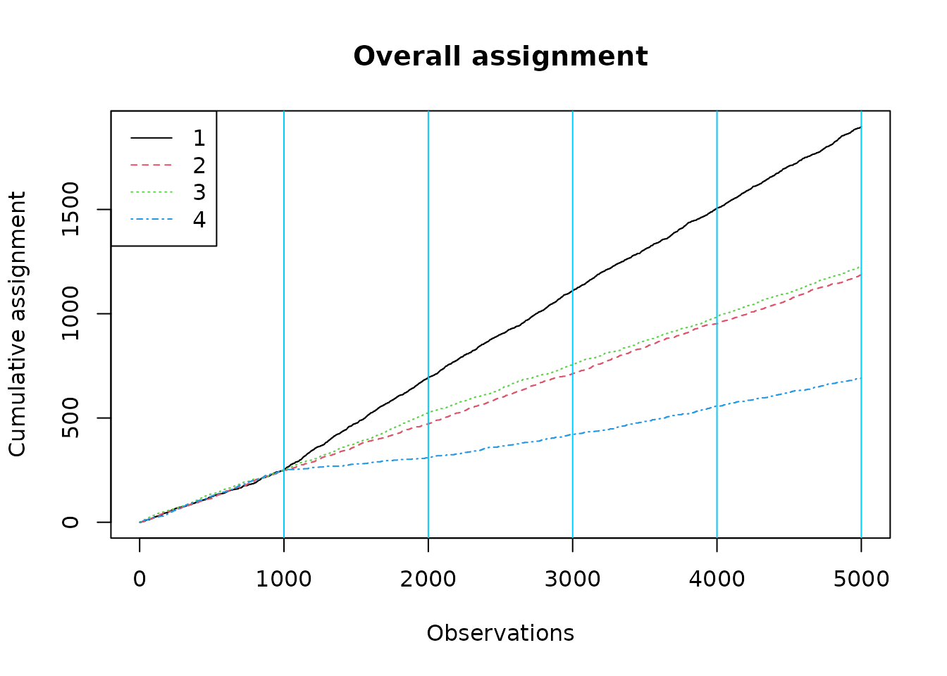
The overall assignment plot over-assigns to the first arm, but we note that our groups are not balanced: the group for whom arm 1 is best is somewhat larger.
muxs <- apply(data[[1]]$muxs, 1, which.max)
cols <- c("#00000080", paste0(palette()[2:4], "4D")) # for transparency
plot(xs[,1], xs[,2], col = cols[muxs], pch = 20, xlab = "X1", ylab = "X2", type = "p",
     cex = 0.5)
graphics::legend("topleft", legend = 1:K, col=1:K, pch=19, title = "Best arm")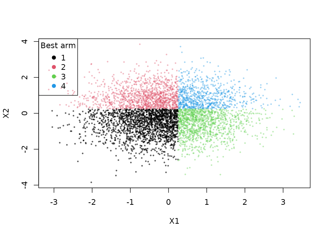
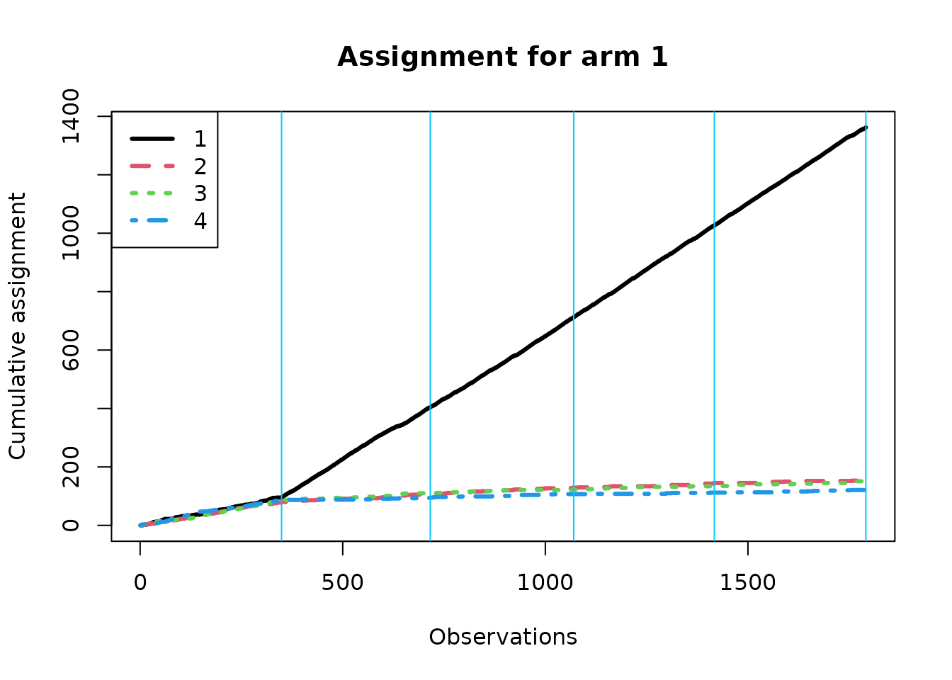
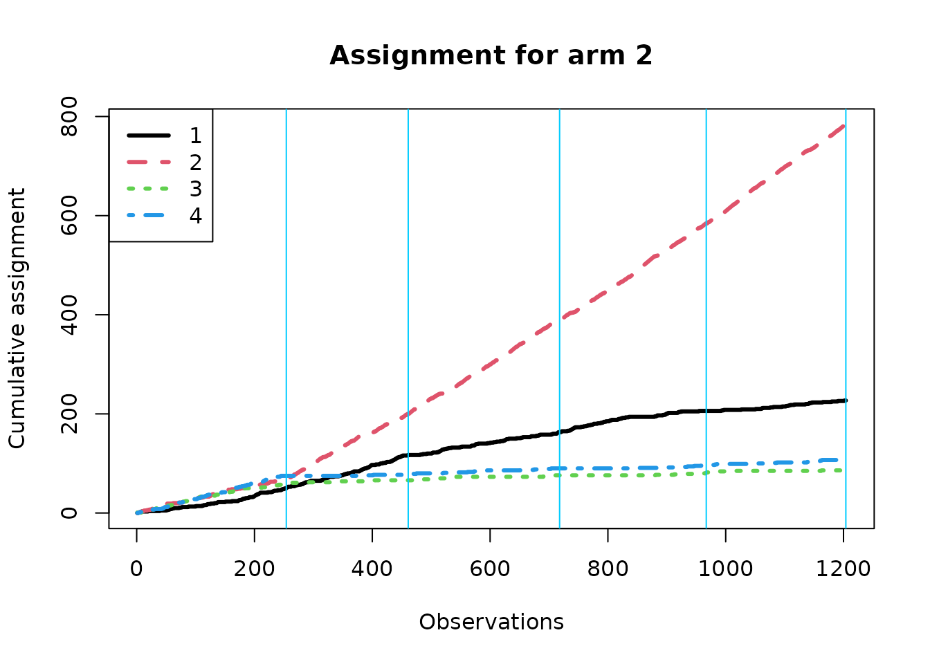
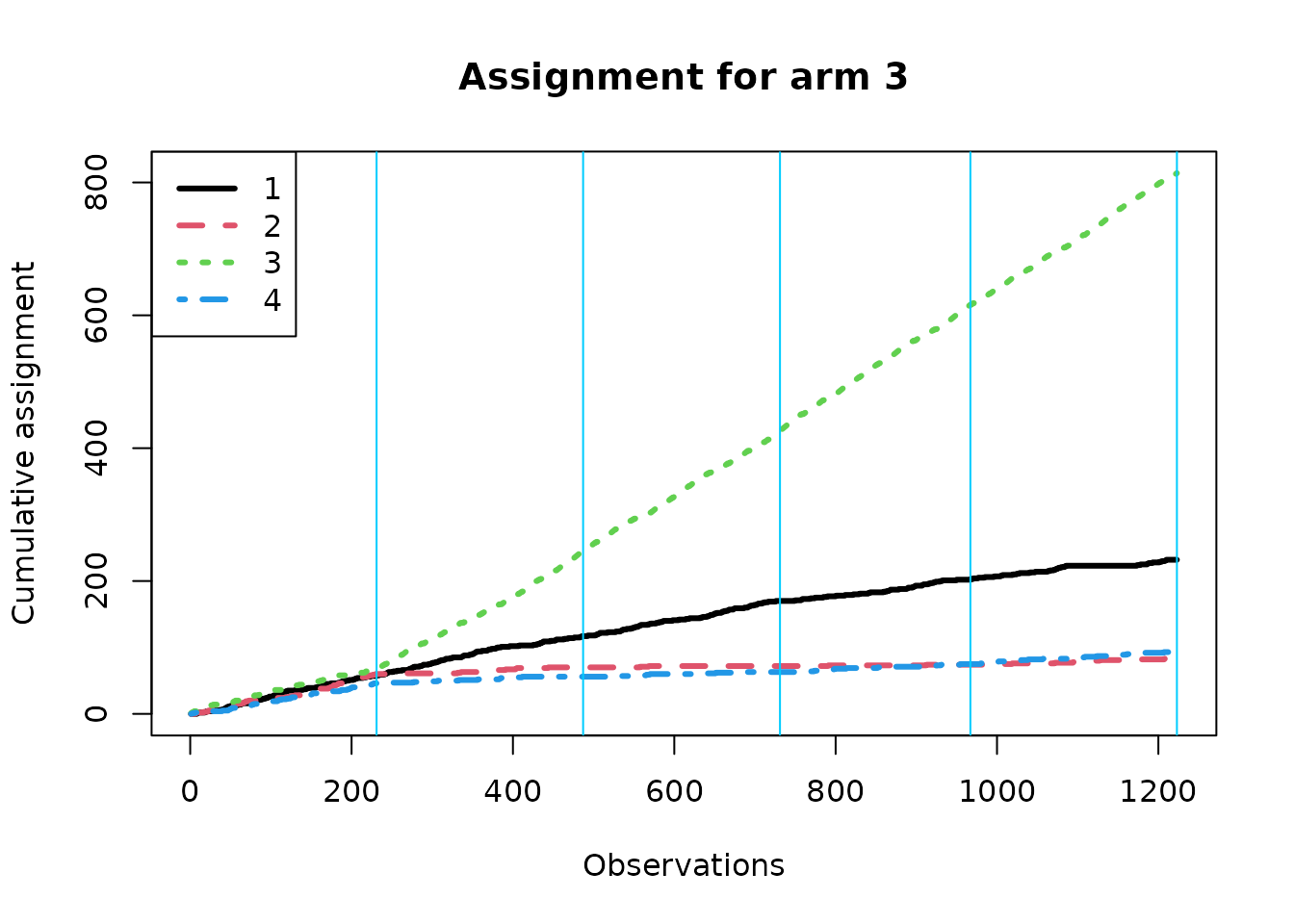
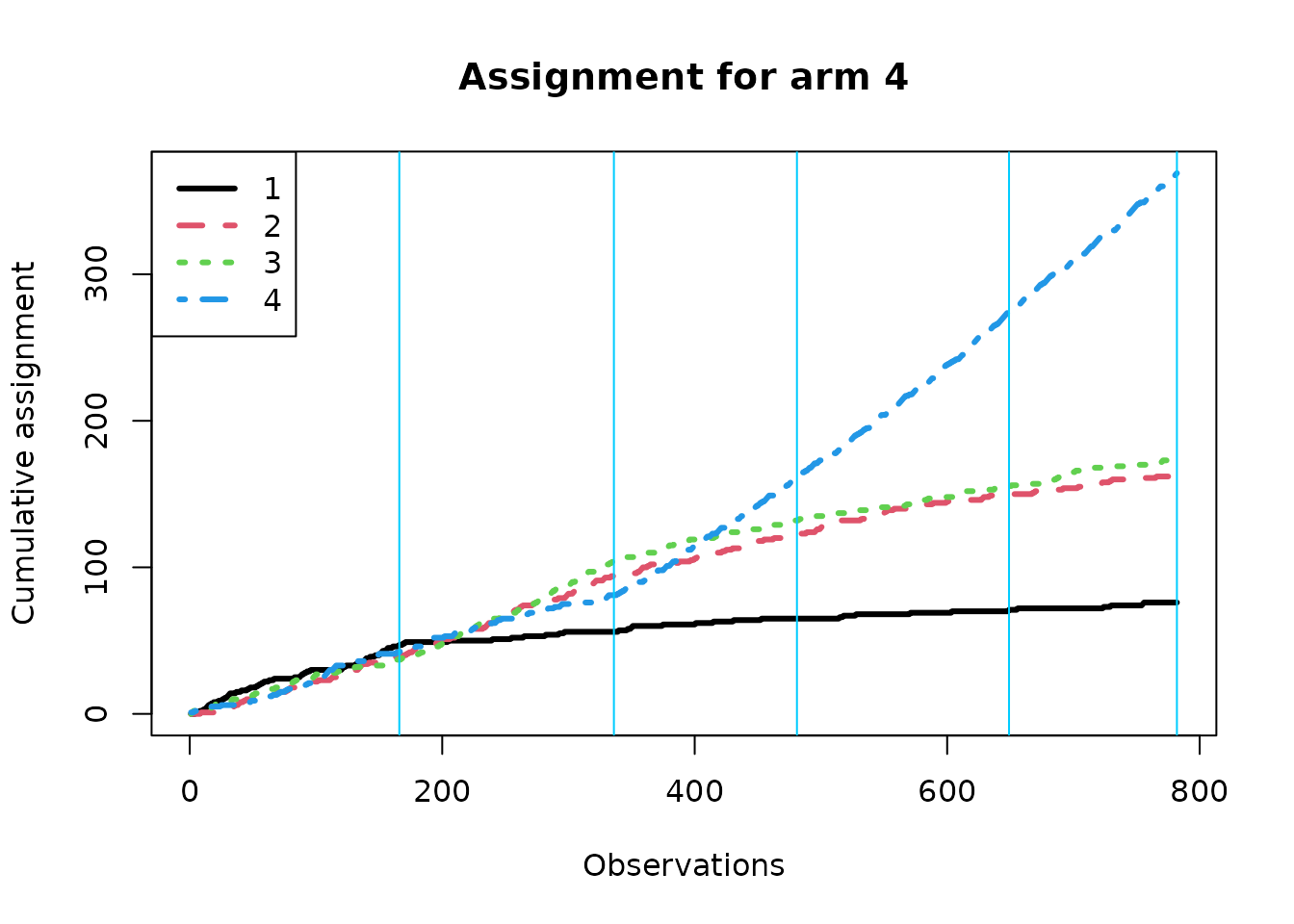
We now create separate assignment plots based on the true best arm; within each context, the algorithm should over-assign treatment to the true best arm if it is learning context correctly. Note that the effective batch sizes are different under the different conditions.
for(k in 1:K){

  idx <- (data[[1]]$muxs[,k]==1)
  batch_sizes_w <- lapply(split(idx, cut(1:sum(batch_sizes),
                                         c(0,cumsum(batch_sizes))) ), sum)

  dat <- matrix(0, nrow = sum(idx), ncol = K)
  dat[cbind(1:sum(idx), results$ws[idx])] <- 1
  dat <- apply(dat, 2, cumsum)
  graphics::matplot(dat, type = c("l"), col =1:K,
                    lwd = 3,
                    xlab = "Observations",
                    ylab = "Cumulative assignment",
                    main = paste0("Assignment for arm ", k))
  graphics::abline(v=cumsum(batch_sizes_w), col="#00ccff")
  graphics::legend("topleft", legend = 1:K, col=1:K, lty=1:K, lwd = 3)

}
Estimating response.
We then generate augmented inverse probability weighted (AIPW)
scores, using a conditional means model and known assignment
probabilities. Here, the conditional means are estimated from a ridge
model, which estimates conditional means for each observation based only
on batchwise history, using the ridge_muhat_lfo_pai()
function. Other conditional means models can also be used.
# Get estimates for policies

# conditional means model
mu_hat <- ridge_muhat_lfo_pai(xs=xs,
                              ws=results$ws,
                              yobs=results$yobs,
                              K=K,
                              batch_sizes=batch_sizes)

# Our conditional means model is currently 3 dimensional, as we estimate
# counterfactuals for each context at each time point.
# Here, we only need the estimate for the actual time point in which the
# observation was realized.
mu_hat2d <- mu_hat[1,,]
for(i in 1:nrow(mu_hat2d)){
  mu_hat2d[i,] <- mu_hat[i,i,]
}

# inverse probability score 1[W_t=w]/e_t(w) of pulling arms, shape [A, K]
balwts <- calculate_balwts(results$ws, results$probs)


# Putting it together, generate doubly robust scores
aipw_scores <- aw_scores(
  ws = results$ws,
  yobs = results$yobs,
  mu_hat = mu_hat2d,
  K = ncol(results$ys),
  balwts = balwts)

## Define counterfactual policies
### Control policy matrix policy0. This is a matrix with A rows and K columns,
### where the elements in the first column are all 1s and the elements in the
## remaining columns are all 0s.
policy0 <- matrix(0, nrow = A, ncol = K)
policy0[,1] <- 1

### Treatment policies list policy1. This is a list with K elements, where each
### list contains a matrix with A rows and K columns. Identifier of treatment x:
### the x th column of the matrix in the x th policy in the list is 1.
policy1 <- lapply(1:K, function(x) {
  pol_mat <- matrix(0, nrow = A, ncol = K)
  pol_mat[,x] <- 1
  pol_mat
}
)

## Estimating the value Q(w) of a single arm w. Here we estimate all the arms in
## policy1 in turn.
out_full <- output_estimates(
  policy1 = policy1,
  gammahat = aipw_scores,
  probs_array = results$probs,
  floor_decay = 0)
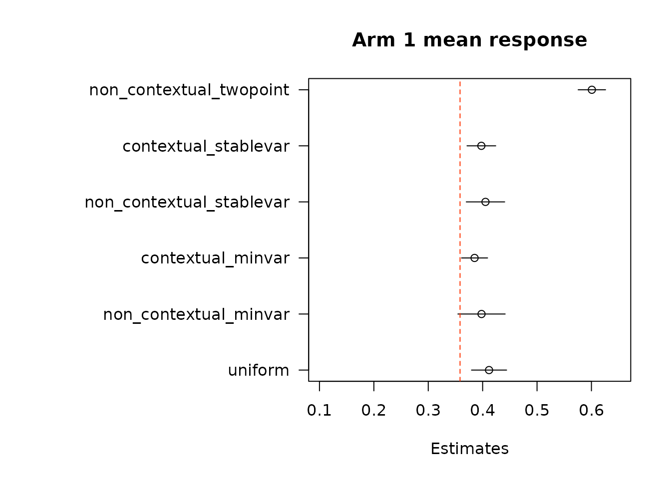
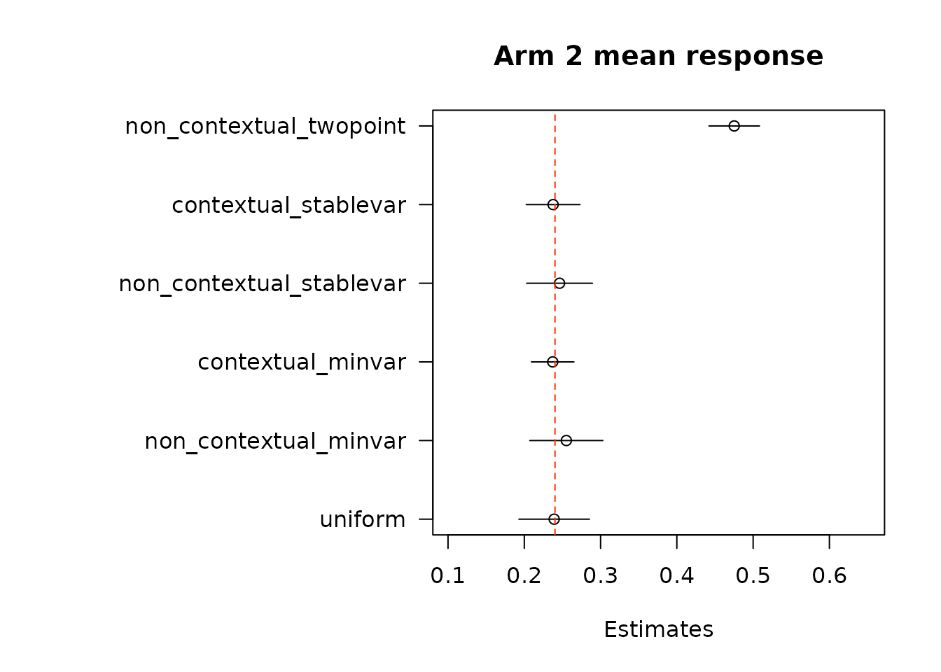
We first look at estimates of mean response under each of the treatment arms. True mean values are represented by the dashed red line.
op <- par(no.readonly = TRUE)

par(mar = c(5,16,4,2) + 0.1)

# set some plotting parameters across plots
xmin <- min(unlist(lapply(out_full, `[`, TRUE, "estimate")), na.rm = TRUE) -
  2* max(unlist(lapply(out_full, `[`, TRUE, "std.error")), na.rm = TRUE)
xmax <- max(unlist(lapply(out_full, `[`, TRUE, "estimate")), na.rm = TRUE) +
  2* max(unlist(lapply(out_full, `[`, TRUE, "std.error")), na.rm = TRUE)

for(i in 1:length(out_full)){
  xest <- out_full[[i]][,"estimate"]
  x0 <- out_full[[i]][,"estimate"] - 1.96*out_full[[i]][,"std.error"]
  x1 <- out_full[[i]][,"estimate"] + 1.96*out_full[[i]][,"std.error"]
  margin <- 2*mean(out_full[[i]][,"std.error"])

  plot(x = xest,
       y = 1:length(xest),
       yaxt = "n",
       xlab = "Estimates",
       ylab = "",
       xlim = c(xmin,
                xmax),
       main = paste0("Arm ", i, " mean response"))
  segments(y0 = 1:length(xest),
           y1 = 1:length(xest),
           x0 = x0,
           x1 = x1)
  axis(2, at = 1:length(xest),
       labels = names(xest), las = 2)
  abline(v = data$mus[i], col = "#FF3300", lty = "dashed")

}
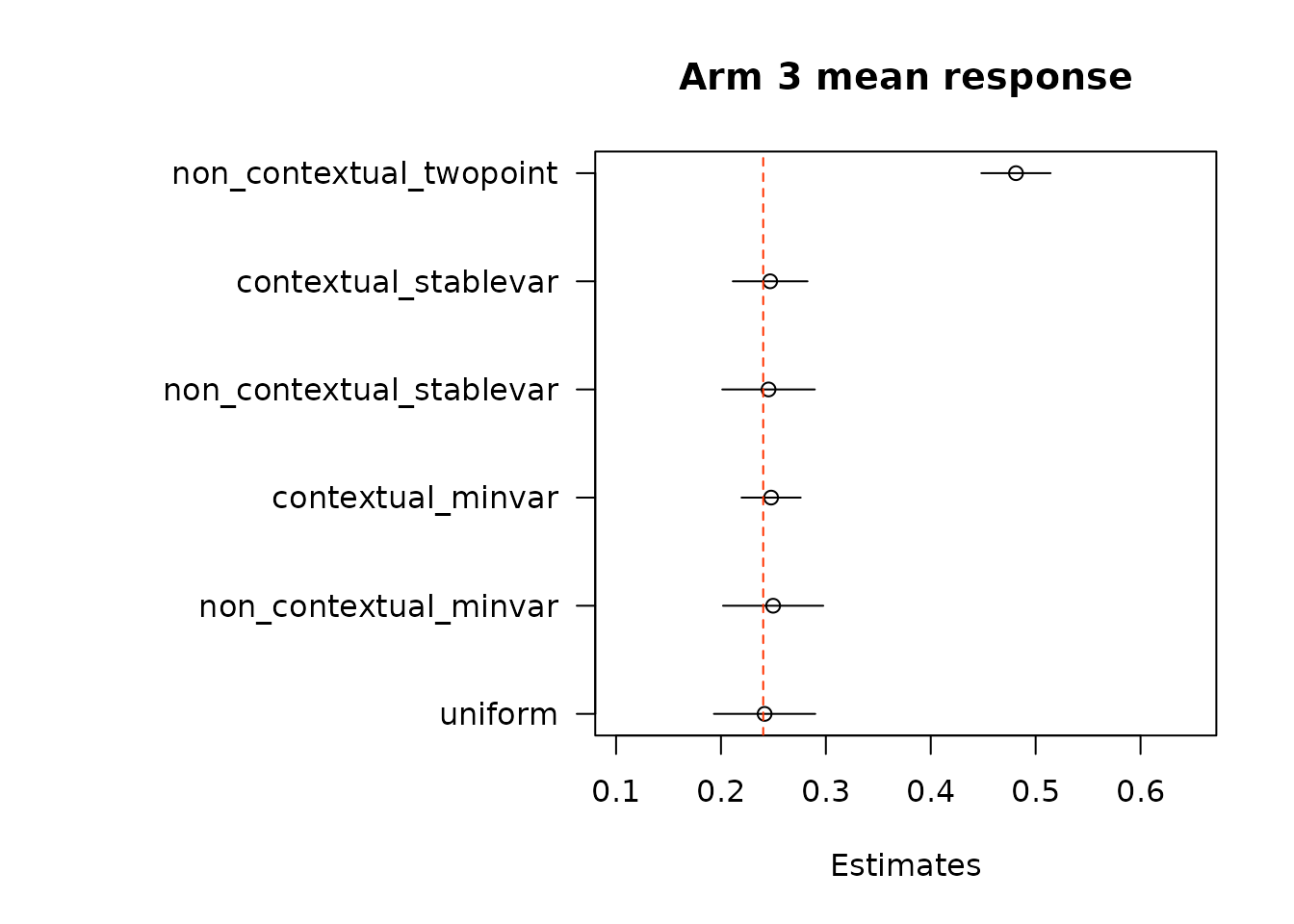
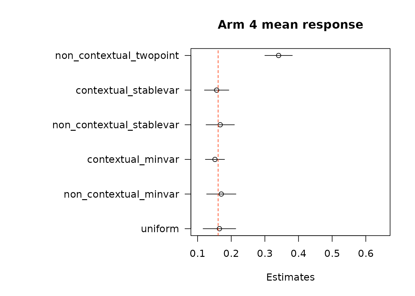
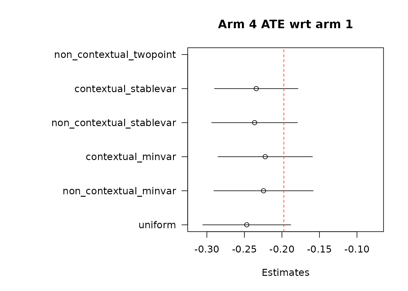
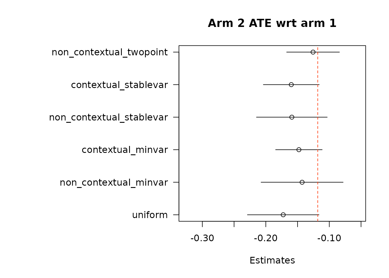
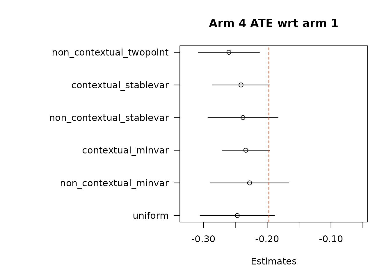
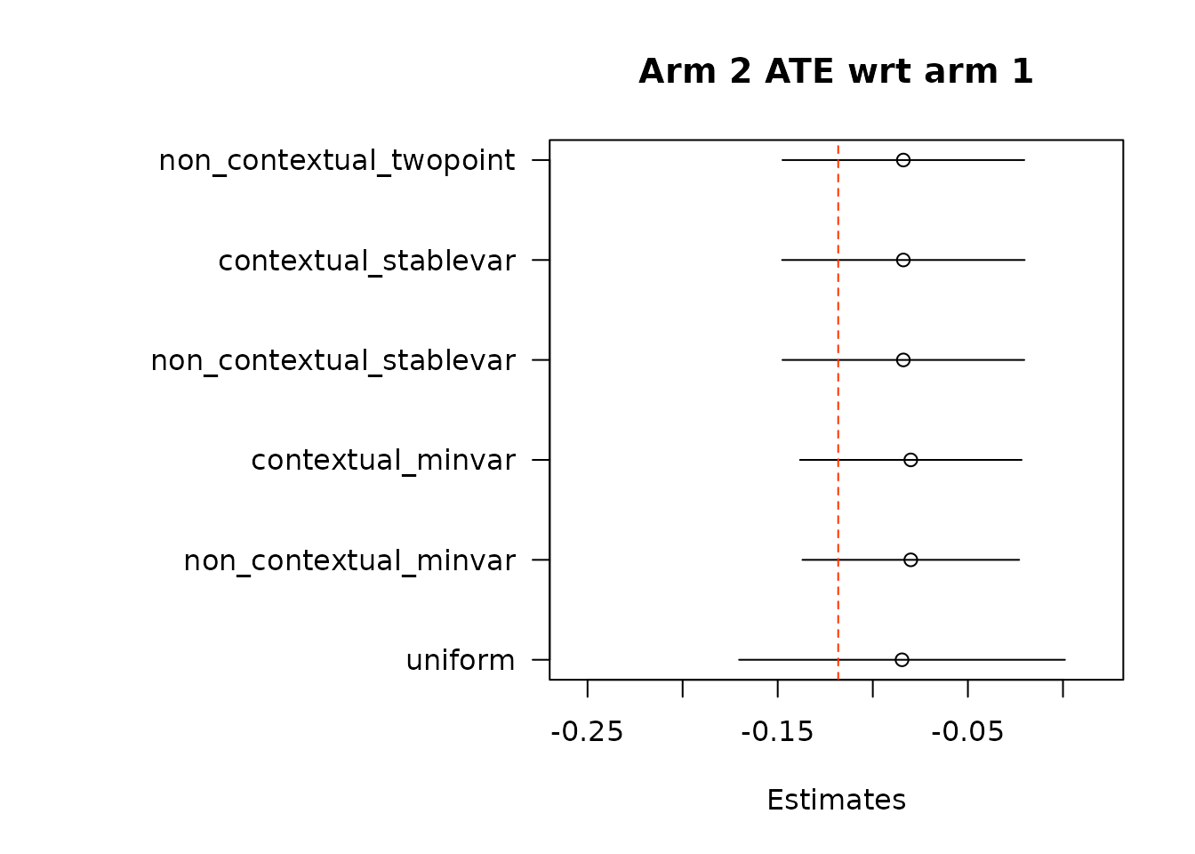
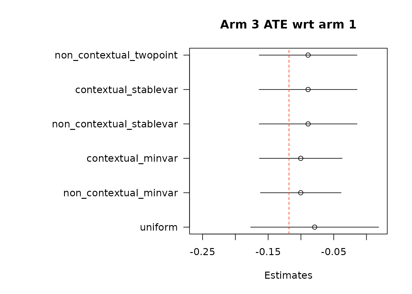
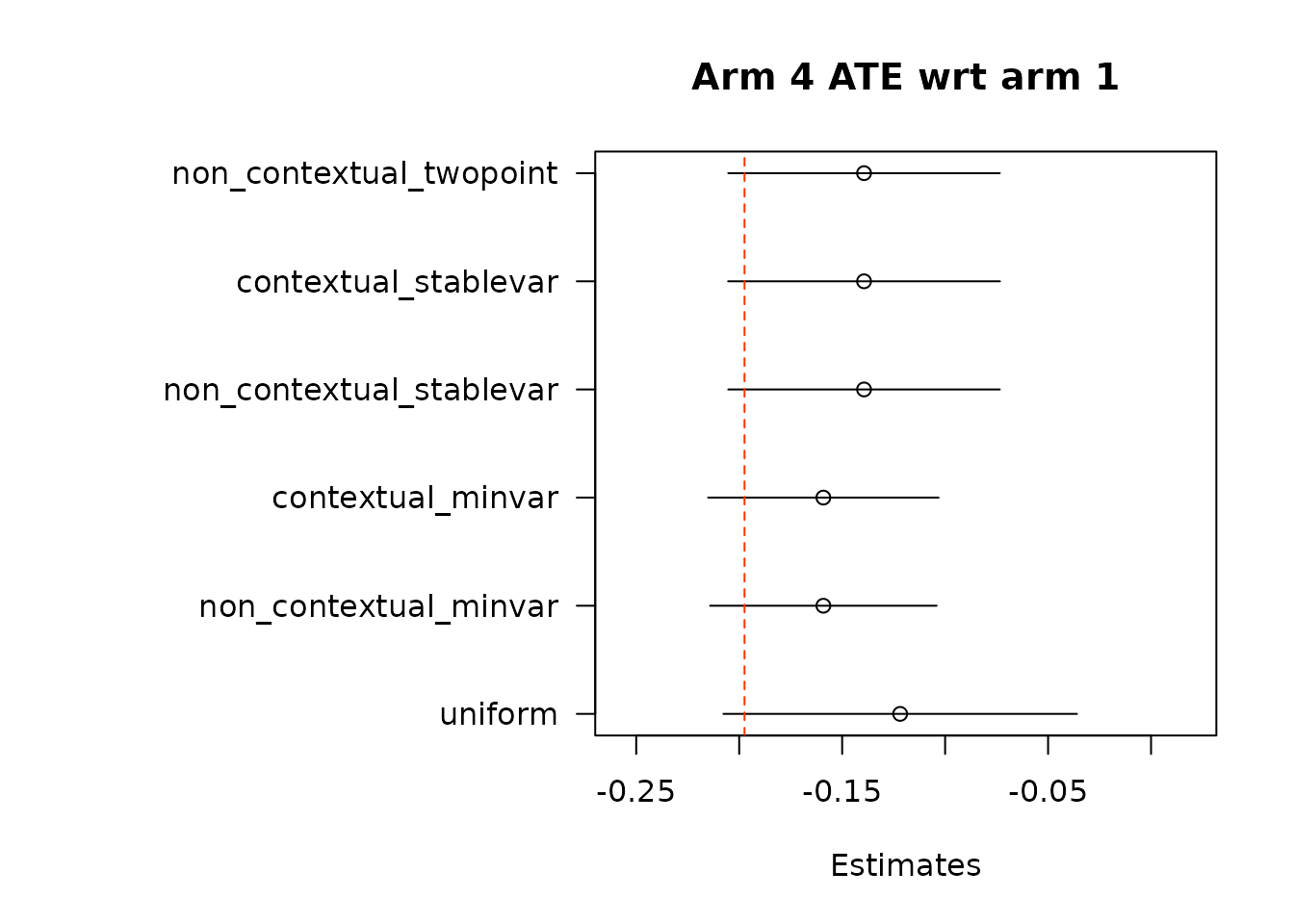
suppressWarnings(par(op))Then, we estimate average treatment effects of each arm compared to the control arm, arm 1, using two different methods.
# Get estimates for treatment effects of policies in contrast to control
# \delta(w_1, w_2) = E[Y_t(w_1) - Y_t(w_2)].
# In Hadad et al. (2021) there are two approaches.
## The first approach: use the difference in AIPW scores as the unbiased scoring
## rule for \delta (w_1, w_2)
### The following function implements the first approach by subtracting policy0,
### the control arm, from all the arms in policy1, except for the control arm
### itself.
out_full_te1 <- output_estimates(
  policy0 = policy0,
  policy1 = policy1[-1],  ## remove the control arm from policy1
  contrasts = "combined",
  gammahat = aipw_scores,
  probs_array = results$probs,
  floor_decay = 0,
  non_contextual_twopoint = FALSE)

## The second approach takes asymptotically normal inference about
## \delta(w_1, w_2): \delta ^ hat (w_1, w_2) = Q ^ hat (w_1) - Q ^ hat (w_2)
out_full_te2 <- output_estimates(
  policy0 = policy0,
  policy1 = policy1[-1],  ## remove the control arm from policy1
  contrasts = "separate",
  gammahat = aipw_scores,
  probs_array = results$probs,
floor_decay = 0)- Under the first approach, we calculate AIPW scores under both treatment(s) and control, take the difference in AIPW scores, and then conduct adaptive weighting.
Note: We do not used this combined estimation method with the non-contextual two-point estimation approach, which produces unstable estimates, and is not supported in the original source. We can do non-contextual two-point estimation when calculating separate adaptive weights for contrasts, however we recommend using other estimation procedures in contextual adaptive settings.
par(mar = c(5,16,4,2) + 0.1)

# set some plotting parameters across plots
xmin <- min(unlist(lapply(out_full_te1, `[`, TRUE, "estimate")), na.rm = TRUE) -
  2* max(unlist(lapply(out_full_te1, `[`, TRUE, "std.error")), na.rm = TRUE)
xmax <- max(unlist(lapply(out_full_te1, `[`, TRUE, "estimate")), na.rm = TRUE) +
  2* max(unlist(lapply(out_full_te1, `[`, TRUE, "std.error")), na.rm = TRUE)

for(i in 1:length(out_full_te1)){
  xest <- out_full_te1[[i]][,"estimate"]
  x0 <- out_full_te1[[i]][,"estimate"] - 1.96*out_full_te1[[i]][,"std.error"]
  x1 <- out_full_te1[[i]][,"estimate"] + 1.96*out_full_te1[[i]][,"std.error"]
  margin <- 2*mean(out_full_te1[[i]][,"std.error"])

  plot(x = xest,
       y = 1:length(xest),
       yaxt = "n",
       xlab = "Estimates",
       ylab = "",
       xlim = c(xmin,
                xmax),
       main = paste0("Arm ", i+1, " ATE wrt arm 1"))
  segments(y0 = 1:length(xest),
           y1 = 1:length(xest),
           x0 = x0,
           x1 = x1)
  axis(2, at = 1:length(xest),
       labels = names(xest), las = 2)
  abline(v = data$mus[i+1] - data$mus[1], col = "#FF3300", lty = "dashed")

}

suppressWarnings(par(op))- In the second approach, we implement adaptive weighting on treatment and control scores separately, and then take the difference.
par(mar = c(5,16,4,2) + 0.1)

# set some plotting parameters across plots
xmin <- min(unlist(lapply(out_full_te2, `[`, TRUE, "estimate")), na.rm = TRUE) -
  2* max(unlist(lapply(out_full_te2, `[`, TRUE, "std.error")), na.rm = TRUE)
xmax <- max(unlist(lapply(out_full_te2, `[`, TRUE, "estimate")), na.rm = TRUE) +
  2* max(unlist(lapply(out_full_te2, `[`, TRUE, "std.error")), na.rm = TRUE)

for(i in 1:length(out_full_te2)){
  xest <- out_full_te2[[i]][,"estimate"]
  x0 <- out_full_te2[[i]][,"estimate"] - 1.96*out_full_te2[[i]][,"std.error"]
  x1 <- out_full_te2[[i]][,"estimate"] + 1.96*out_full_te2[[i]][,"std.error"]
  margin <- 2*mean(out_full_te2[[i]][,"std.error"])

  plot(x = xest,
       y = 1:length(xest),
       yaxt = "n",
       xlab = "Estimates",
       ylab = "",
       xlim = c(xmin,
                xmax),
       main = paste0("Arm ", i+1, " ATE wrt arm 1"))
  segments(y0 = 1:length(xest),
           y1 = 1:length(xest),
           x0 = x0,
           x1 = x1)
  axis(2, at = 1:length(xest),
       labels = names(xest), las = 2)
  abline(v = data$mus[i+1] - data$mus[1], col = "#FF3300", lty = "dashed")

}

par(op)For the non-contextual case.
We also run a non-contextual experiment, using the same original data. The algorithm used is Thompson sampling, without contexts.
# For a noncontextual experiment, we simply omit the context argument
results <- run_experiment(ys = ys,
                          floor_start = 0.025,
                          floor_decay = 0,
                          batch_sizes = batch_sizes)

# plot the cumulative assignment graph
# x-axis is the number of observations, y-axis is the cumulative assignment
plot_cumulative_assignment(results, batch_sizes)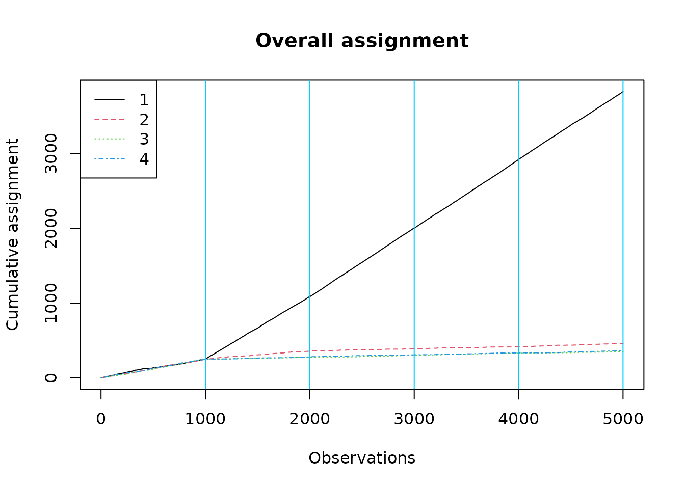
Estimating response.
# Get estimates for policies
# inverse probability score 1[W_t=w]/e_t(w) of pulling arms, shape [A, K]
balwts <- calculate_balwts(results$ws, results$probs)

# Generate doubly robust scores; we don't use the contexts for a means model
# here, but we could, even though they are not used in assignment.
aipw_scores <- aw_scores(
  ws = results$ws,
  yobs = results$yobs,
  K = ncol(results$ys),
  balwts = balwts)

## Define counterfactual policies
### Control policy matrix policy0. This is a matrix with A rows and K columns,
### where the elements in the first column are all 1s and the elements in the
## remaining columns are all 0s.
policy0 <- matrix(0, nrow = A, ncol = K)
policy0[,1] <- 1

### Treatment policies list policy1. This is a list with K elements, where each
### list contains a matrix with A rows and K columns. Identifier of treatment x:
### the x th column of the matrix in the x th policy in the list is 1.
policy1 <- lapply(1:K, function(x) {
  pol_mat <- matrix(0, nrow = A, ncol = K)
  pol_mat[,x] <- 1
  pol_mat
}
)

## Estimating the value Q(w) of a single arm w. Here we estimate all the arms in
## policy1 in turn.
out_full <- output_estimates(
  policy1 = policy1,
  gammahat = aipw_scores,
  probs_array = results$probs,
  floor_decay = 0)
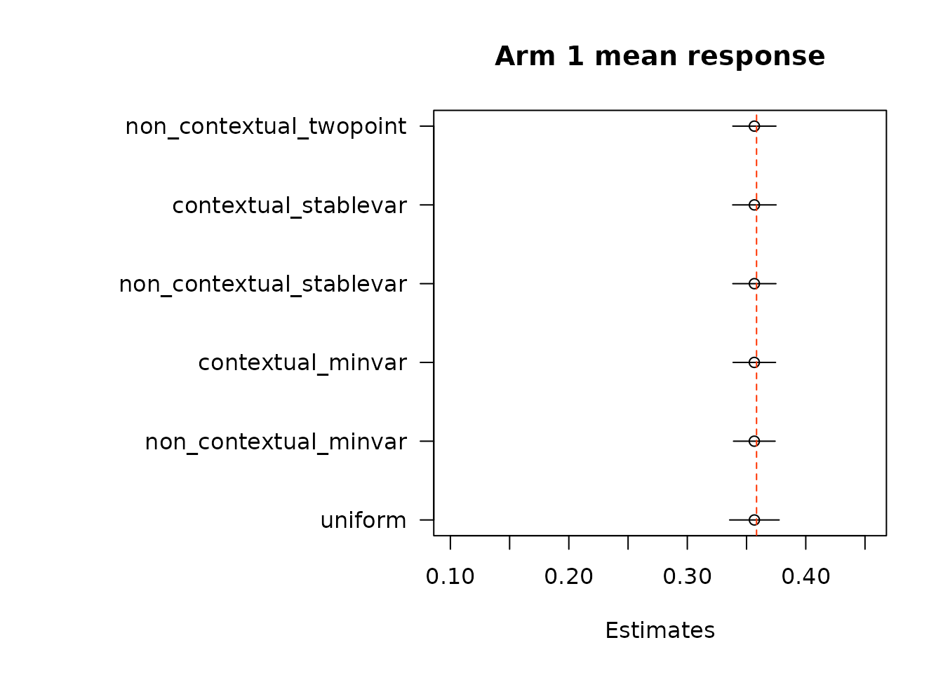
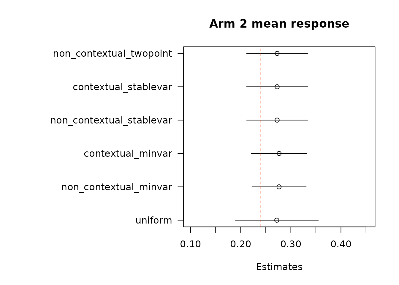
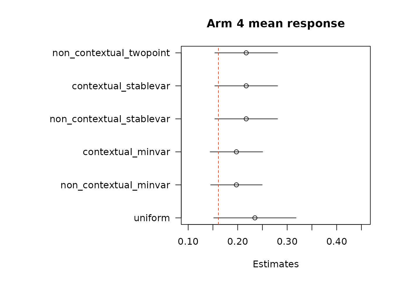
We first look at estimates of mean response under each of the treatment arms. True mean values are represented by the dashed red line.
par(mar = c(5,16,4,2) + 0.1)

# set some plotting parameters across plots
xmin <- min(unlist(lapply(out_full, `[`, TRUE, "estimate"))) -
  2* max(unlist(lapply(out_full, `[`, TRUE, "std.error")))
xmax <- max(unlist(lapply(out_full, `[`, TRUE, "estimate"))) +
  2* max(unlist(lapply(out_full, `[`, TRUE, "std.error")))

for(i in 1:length(out_full)){
  xest <- out_full[[i]][,"estimate"]
  x0 <- out_full[[i]][,"estimate"] - 1.96*out_full[[i]][,"std.error"]
  x1 <- out_full[[i]][,"estimate"] + 1.96*out_full[[i]][,"std.error"]
  margin <- 2*mean(out_full[[i]][,"std.error"])

  plot(x = xest,
       y = 1:length(xest),
       yaxt = "n",
       xlab = "Estimates",
       ylab = "",
       xlim = c(xmin,
                xmax),
       main = paste0("Arm ", i, " mean response"))
  segments(y0 = 1:length(xest),
           y1 = 1:length(xest),
           x0 = x0,
           x1 = x1)
  axis(2, at = 1:length(xest),
       labels = names(xest), las = 2)
  abline(v = data$mus[i], col = "#FF3300", lty = "dashed")

}

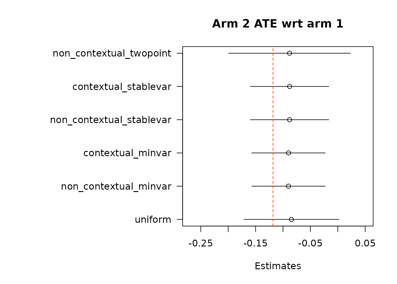
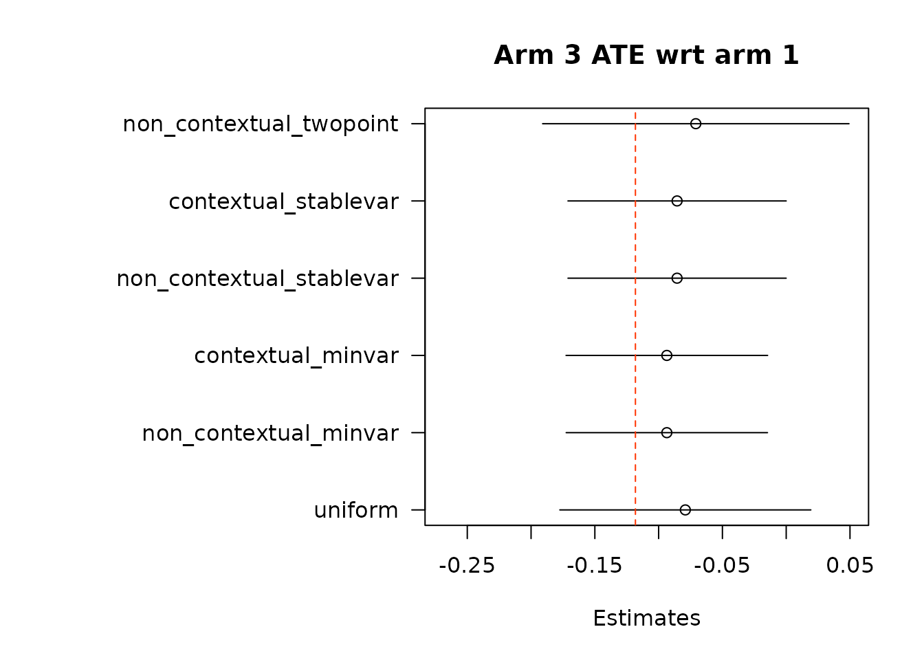
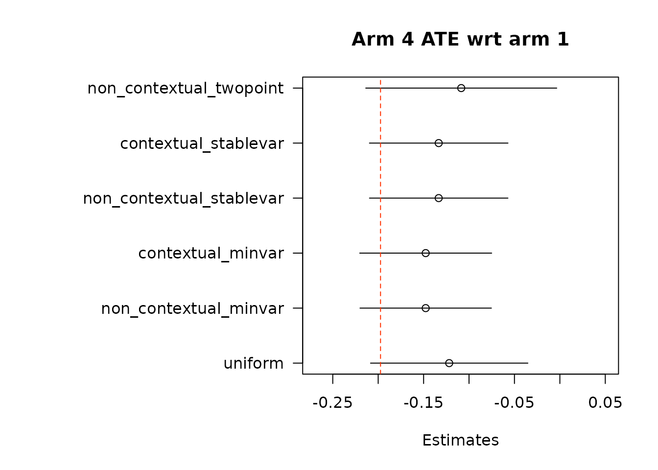
par(op)We again estimate average treatment effects of each arm compared to the control arm, arm 1, using the two different methods.
# Get estimates for treatment effects of policies in contrast to control
# \delta(w_1, w_2) = E[Y_t(w_1) - Y_t(w_2)].
# In Hadad et al. (2021) there are two approaches.
## The first approach: use the difference in AIPW scores as the unbiased scoring
## rule for \delta (w_1, w_2)
### The following function implements the first approach by subtracting policy0,
### the control arm, from all the arms in policy1, except for the control arm
### itself.
out_full_te1 <- output_estimates(
  policy0 = policy0,
  policy1 = policy1[-1],  ## remove the control arm from policy1
  contrasts = "combined",
  gammahat = aipw_scores,
  probs_array = results$probs,
  floor_decay = 0)

## The second approach takes asymptotically normal inference about
## \delta(w_1, w_2): \delta ^ hat (w_1, w_2) = Q ^ hat (w_1) - Q ^ hat (w_2)
out_full_te2 <- output_estimates(
  policy0 = policy0,
  policy1 = policy1[-1],  ## remove the control arm from policy1
  contrasts = "separate",
  gammahat = aipw_scores,
  probs_array = results$probs,
floor_decay = 0)- First take the difference in AIPW scores, and then conduct adaptive weighting.
par(mar = c(5,16,4,2) + 0.1)

# set some plotting parameters across plots
xmin <- min(unlist(lapply(out_full_te1, `[`, TRUE, "estimate")), na.rm = TRUE) -
  2* max(unlist(lapply(out_full_te1, `[`, TRUE, "std.error")), na.rm = TRUE)
xmax <- max(unlist(lapply(out_full_te1, `[`, TRUE, "estimate")), na.rm = TRUE) +
  2* max(unlist(lapply(out_full_te1, `[`, TRUE, "std.error")), na.rm = TRUE)

for(i in 1:length(out_full_te1)){
  xest <- out_full_te1[[i]][,"estimate"]
  x0 <- out_full_te1[[i]][,"estimate"] - 1.96*out_full_te1[[i]][,"std.error"]
  x1 <- out_full_te1[[i]][,"estimate"] + 1.96*out_full_te1[[i]][,"std.error"]
  margin <- 2*mean(out_full_te1[[i]][,"std.error"])

  plot(x = xest,
       y = 1:length(xest),
       yaxt = "n",
       xlab = "Estimates",
       ylab = "",
       xlim = c(xmin,
                xmax),
       main = paste0("Arm ", i+1, " ATE wrt arm 1"))
  segments(y0 = 1:length(xest),
           y1 = 1:length(xest),
           x0 = x0,
           x1 = x1)
  axis(2, at = 1:length(xest),
       labels = names(xest), las = 2)
  abline(v = data$mus[i+1] - data$mus[1], col = "#FF3300", lty = "dashed")

}
suppressWarnings(par(op))- Or implement adaptive weighting on treatment and control scores separately, and then take the difference.
par(mar = c(5,16,4,2) + 0.1)

# set some plotting parameters across plots
xmin <- min(unlist(lapply(out_full_te2, `[`, TRUE, "estimate")), na.rm = TRUE) -
  2* max(unlist(lapply(out_full_te2, `[`, TRUE, "std.error")), na.rm = TRUE)
xmax <- max(unlist(lapply(out_full_te2, `[`, TRUE, "estimate")), na.rm = TRUE) +
  2* max(unlist(lapply(out_full_te2, `[`, TRUE, "std.error")), na.rm = TRUE)

for(i in 1:length(out_full_te2)){
  xest <- out_full_te2[[i]][,"estimate"]
  x0 <- out_full_te2[[i]][,"estimate"] - 1.96*out_full_te2[[i]][,"std.error"]
  x1 <- out_full_te2[[i]][,"estimate"] + 1.96*out_full_te2[[i]][,"std.error"]
  margin <- 2*mean(out_full_te2[[i]][,"std.error"])

  plot(x = xest,
       y = 1:length(xest),
       yaxt = "n",
       xlab = "Estimates",
       ylab = "",
       xlim = c(xmin,
                xmax),
       main = paste0("Arm ", i+1, " ATE wrt arm 1"))
  segments(y0 = 1:length(xest),
           y1 = 1:length(xest),
           x0 = x0,
           x1 = x1)
  axis(2, at = 1:length(xest),
       labels = names(xest), las = 2)
  abline(v = data$mus[i+1] - data$mus[1], col = "#FF3300", lty = "dashed")

}
suppressWarnings(par(op))