library(ggplot2)
library(MASS)
options(digits = 3)1. Probability and Linear Algebra
From random variables to the OLS estimator
This chapter builds up the machinery behind OLS from scratch. We start with expectation and variance, show how the conditional expectation function emerges from a joint distribution, and then shift to linear algebra — matrices, projection, and the geometry that makes regression work.
Questions this chapter answers:
- What is the best predictor of a random variable, and why does the mean minimize squared error?
- How does conditioning on information improve prediction through the CEF?
- How does the design matrix \(\mathbf{X}\) encode a regression problem?
- Why is OLS a geometric projection, and what do eigenvectors of the hat matrix tell us?
1 Expectation as a best guess
If you had to predict a random variable \(Y\) with a single number \(\mu\), and your penalty for being wrong is squared error, you’d choose the mean. Let’s verify this computationally.
Suppose \(Y\) takes values \(\{1, 2, 3, 4, 5\}\) with probabilities \(\{0.1, 0.2, 0.3, 0.25, 0.15\}\).
values <- 1:5
probs <- c(0.1, 0.2, 0.3, 0.25, 0.15)

# The expected value
mu <- sum(values * probs)
mu
[1] 3.15# Mean squared error as a function of the guess
mse <- function(guess) {
sum(probs * (values - guess)^2)
}
# Evaluate over a grid
guesses <- seq(1, 5, by = 0.01)
errors <- sapply(guesses, mse)
ggplot(data.frame(guess = guesses, mse = errors), aes(guess, mse)) +
geom_line(linewidth = 0.8) +
geom_vline(xintercept = mu, linetype = "dashed", color = "steelblue") +
annotate("text", x = mu + 0.3, y = max(errors) * 0.9,
label = paste("E[Y] =", mu), color = "steelblue") +
labs(x = "Guess (mu)", y = "Mean Squared Error",
title = "The expectation minimizes mean squared prediction error") +
theme_minimal()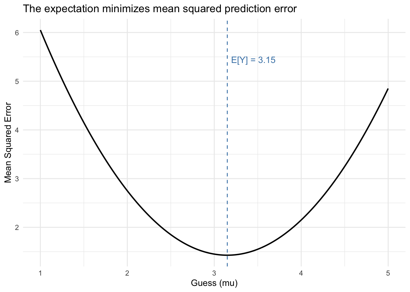
The minimum of the parabola lands exactly at \(\mathbb{E}[Y]\). This is the simplest version of a result that recurs throughout the course: the conditional expectation function minimizes MSE given information.
Theorem 1 (E[Y] Minimizes MSE) Among all constants \(\mu\), the expected value \(\mathbb{E}[Y]\) uniquely minimizes the mean squared error \(\mathbb{E}[(Y - \mu)^2]\).
2 Variance and the deviation identity
Variance measures the average squared distance from the mean:
\[\text{Var}(X) = \mathbb{E}[(X - \mathbb{E}[X])^2] = \mathbb{E}[X^2] - (\mathbb{E}[X])^2 \tag{1}\]
Let’s verify both formulas give the same answer.
EY <- sum(values * probs)
EY2 <- sum(values^2 * probs)

# Definition form
var_def <- sum(probs * (values - EY)^2)

# Shortcut form
var_short <- EY2 - EY^2

c(definition = var_def, shortcut = var_short)
definition shortcut
1.43 1.43 In a sample, we can also write the variance as \(\frac{1}{n}\sum(x_i - \bar{x})x_i\). This works because deviations from the mean always sum to zero: \(\sum(x_i - \bar{x}) = 0\), so shifting the second factor by any constant changes nothing. This same algebra produces the OLS normal equations later.
The interactive visualization below makes this concrete using the sample \(x = \{1, 5, 6, 8\}\) with mean \(\bar{x} = 5\). Think of each term as the signed area of a rectangle with width \((x_i - \bar{x})\) and height \((x_i - c)\). Slide \(c\) from \(\bar{x}\) down to \(0\): the rectangles change shape, but the total signed area stays constant.
3 Joint distributions and the CEF
The lecture works through an example where two parties (A and B) mobilize voters, with joint density \(f(x, y) = 6(1 - x - y)\) for \(x, y \geq 0\) and \(x + y \leq 1\). Let’s visualize this and compute the CEF.
# Create a grid
grid <- expand.grid(x = seq(0, 1, length = 200), y = seq(0, 1, length = 200))
grid$density <- ifelse(grid$x + grid$y <= 1,
                       6 * (1 - grid$x - grid$y), NA)

ggplot(grid, aes(x, y, fill = density)) +
  geom_tile() +
  scale_fill_viridis_c(na.value = "white", name = "f(x,y)") +
  labs(title = "Joint density: f(x, y) = 6(1 - x - y)",
       x = "Party A mobilization (x)",
       y = "Party B mobilization (y)") +
  coord_fixed() +
  theme_minimal()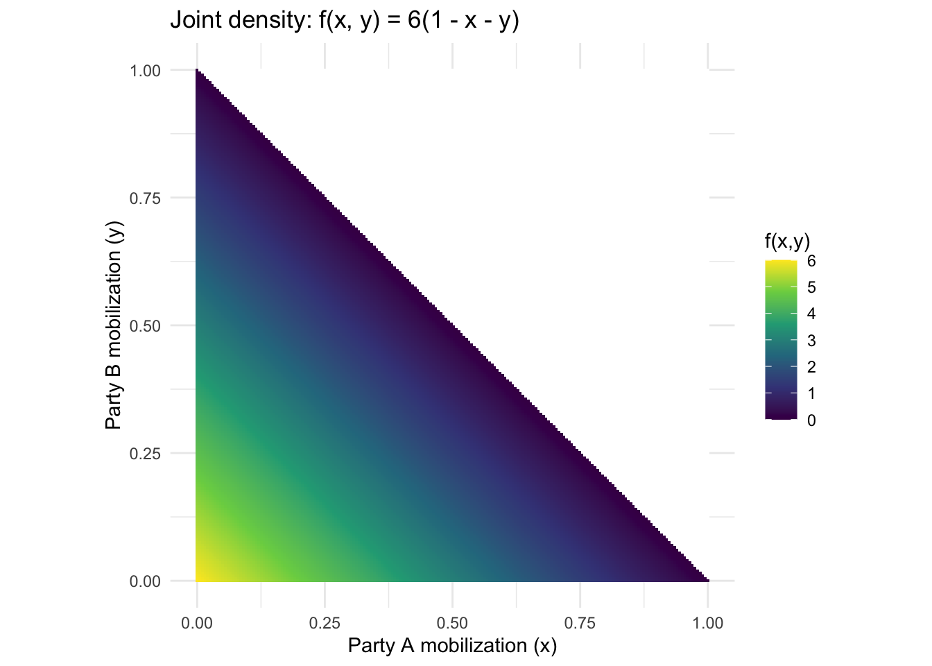
From the joint density we can derive the marginal \(f_X(x) = 3(1-x)^2\), the conditional \(f_{Y|X}(y|x) = \frac{2(1-x-y)}{(1-x)^2}\), and the CEF \(\mathbb{E}[Y|X=x] = \frac{1-x}{3}\). Let’s verify by simulation.
# Simulate from f(x,y) = 6(1-x-y) using rejection sampling
set.seed(123)
n_sim <- 50000
samples <- data.frame(x = numeric(0), y = numeric(0))

while (nrow(samples) < n_sim) {
  x_prop <- runif(n_sim)
  y_prop <- runif(n_sim)
  valid <- (x_prop + y_prop <= 1)
  x_prop <- x_prop[valid]
  y_prop <- y_prop[valid]
  # Accept with probability proportional to density
  accept_prob <- 6 * (1 - x_prop - y_prop) / 6  # max density is 6

  keep <- runif(length(x_prop)) < accept_prob
  samples <- rbind(samples, data.frame(x = x_prop[keep], y = y_prop[keep]))
}
samples <- samples[1:n_sim, ]

# Bin x and compute mean of y in each bin
samples$x_bin <- cut(samples$x, breaks = 30)
cef_empirical <- aggregate(y ~ x_bin, data = samples, FUN = mean)
cef_empirical$x_mid <- seq(0.02, 0.98, length = nrow(cef_empirical))

# Plot simulation vs. theoretical CEF
ggplot(cef_empirical, aes(x_mid, y)) +
  geom_point(alpha = 0.7) +
  stat_function(fun = function(x) (1 - x) / 3, color = "red", linewidth = 1) +
  labs(x = "x", y = "E[Y | X = x]",
       title = "CEF: simulation vs. theory",
       subtitle = "Red line: (1 - x)/3") +
  theme_minimal()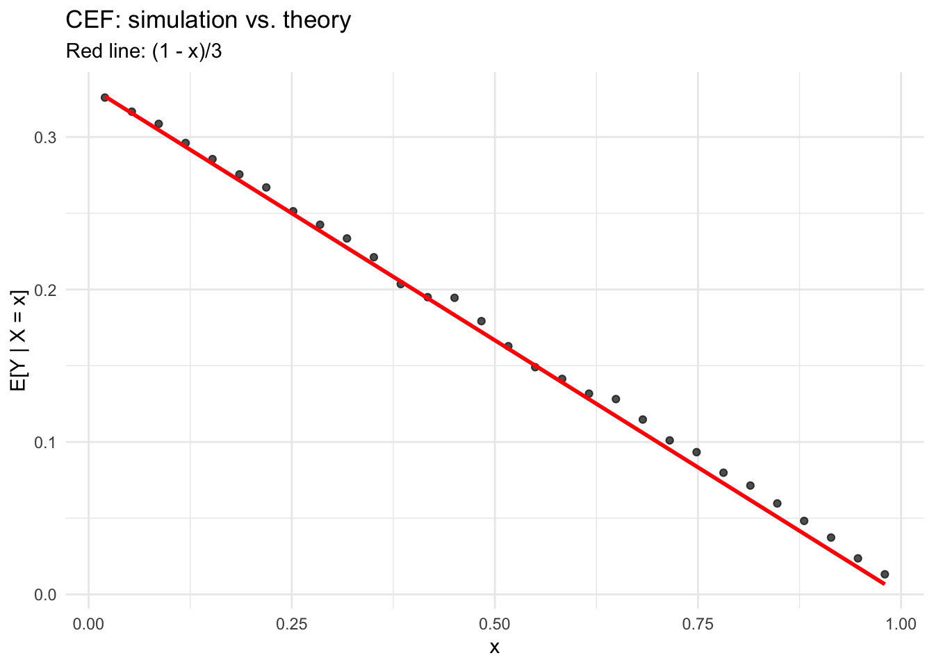
The simulated conditional means track the theoretical CEF closely. This is a case where the CEF happens to be linear — but that’s a special property of this density, not a general fact.
4 The law of iterated expectations
The LIE says \(\mathbb{E}[\mathbb{E}[Y|X]] = \mathbb{E}[Y]\). In words: the average of the conditional averages equals the overall average. Let’s check.
# Overall mean of Y from simulation
overall_mean <- mean(samples$y)

# Theoretical E[Y]: integrate y * f_Y(y)
# f_Y(y) = 3(1-y)^2 by symmetry, so E[Y] = integral of y * 3(1-y)^2 from 0 to 1
EY_theory <- integrate(function(y) y * 3 * (1 - y)^2, 0, 1)$value

# E[E[Y|X]] = E[(1-X)/3] = integral of (1-x)/3 * 3(1-x)^2 dx = integral of (1-x)^3 dx
EEY_X <- integrate(function(x) (1 - x)^3, 0, 1)$value

c(simulation = overall_mean, `E[Y] theory` = EY_theory, `E[E[Y|X]]` = EEY_X)
simulation E[Y] theory E[E[Y|X]]
0.25 0.25 0.25 All three agree: the LIE holds.
Theorem 2 (Law of Iterated Expectations) For any random variables \(X\) and \(Y\), \(\mathbb{E}[\mathbb{E}[Y|X]] = \mathbb{E}[Y]\). The average of the conditional averages equals the unconditional average.
5 Law of total variance
The law of total variance decomposes \(\text{Var}(Y) = \mathbb{E}[\text{Var}(Y|X)] + \text{Var}(\mathbb{E}[Y|X])\). This is the foundation of \(R^2\).
# Var(Y) from simulation
var_y_sim <- var(samples$y)

# Compute within each bin: variance of y and mean of y
bin_stats <- aggregate(y ~ x_bin, data = samples, FUN = function(z) c(m = mean(z), v = var(z), n = length(z)))
bin_stats <- do.call(data.frame, bin_stats)

# E[Var(Y|X)] - average of conditional variances (weighted by bin size)
weights <- bin_stats$y.n / sum(bin_stats$y.n)
E_var_YX <- sum(weights * bin_stats$y.v)

# Var(E[Y|X]) - variance of conditional means
var_EYX <- sum(weights * (bin_stats$y.m - sum(weights * bin_stats$y.m))^2)

c(`Var(Y)` = var_y_sim,
  `E[Var(Y|X)] + Var(E[Y|X])` = E_var_YX + var_EYX,
  `explained fraction` = var_EYX / var_y_sim)
Var(Y) E[Var(Y|X)] + Var(E[Y|X]) explained fraction
0.0375 0.0375 0.1125 The decomposition works. The “explained fraction” is essentially \(R^2\): how much of the total variance of \(Y\) is captured by the CEF.
Theorem 3 (Law of Total Variance) \(\text{Var}(Y) = \mathbb{E}[\text{Var}(Y|X)] + \text{Var}(\mathbb{E}[Y|X])\). Total variance decomposes into average conditional variance plus variance of conditional means.
6 From probability to matrices
Now we shift gears. The CEF tells us what we’re trying to estimate. Linear algebra tells us how.
6.1 The design matrix
In regression, we organize our data as \(\mathbf{y} = \mathbf{X}\boldsymbol{\beta} + \mathbf{e}\). Let’s build a design matrix and see what \(\mathbf{X}'\mathbf{X}\) and \(\mathbf{X}'\mathbf{y}\) look like.
set.seed(2026)
n <- 50
x1 <- rnorm(n)
x2 <- rnorm(n)
y <- 2 + 3 * x1 - 1.5 * x2 + rnorm(n)

# Build the design matrix (intercept + two regressors)
X <- cbind(1, x1, x2)
colnames(X) <- c("intercept", "x1", "x2")
head(X)
intercept x1 x2
[1,] 1 0.5206 -1.170
[2,] 1 -1.0797 -0.206
[3,] 1 0.1392 -0.931
[4,] 1 -0.0847 0.449
[5,] 1 -0.6666 -0.645
[6,] 1 -2.5161 -0.2316.2 The Gram matrix \(\mathbf{X}'\mathbf{X}\)
This matrix encodes all second-moment information about the regressors. Its \((i,j)\) entry is the inner product of columns \(i\) and \(j\).
XtX <- t(X) %*% X
XtX
intercept x1 x2
intercept 50.000 -0.813 -8.99
x1 -0.813 46.685 11.93
x2 -8.991 11.926 53.88# It's symmetric
all.equal(XtX, t(XtX))[1] TRUE# And positive definite (all eigenvalues positive)
eigen(XtX)$values[1] 66.5 48.1 36.0All eigenvalues are positive, so \(\mathbf{X}'\mathbf{X}\) is positive definite and invertible.
NoteFull Rank Assumption
OLS requires \(\mathbf{X}'\mathbf{X}\) to be invertible, which holds when \(\mathbf{X}\) has full column rank — no column is a perfect linear combination of others. Equivalently, all eigenvalues of \(\mathbf{X}'\mathbf{X}\) must be strictly positive.
6.3 Computing OLS by hand
The OLS estimator is \(\hat{\boldsymbol{\beta}} = (\mathbf{X}'\mathbf{X})^{-1}\mathbf{X}'\mathbf{y}\). Let’s compute it step by step.
Xty <- t(X) %*% y
beta_hat <- solve(XtX) %*% Xty

# Compare to lm()
beta_lm <- coef(lm(y ~ x1 + x2))

cbind(manual = beta_hat, lm = beta_lm)
lm
intercept 2.13 2.13
x1 2.93 2.93
x2 -1.50 -1.50They match. The solve() function computes the matrix inverse, and %*% does matrix multiplication.
TipUse
crossprod() for Speed
crossprod(X) computes \(X'X\) more efficiently than t(X) %*% X, and crossprod(X, y) computes \(X'y\). For large matrices, the speedup is substantial.
7 Projection and residuals
OLS is a projection. The hat matrix \(\mathbf{P} = \mathbf{X}(\mathbf{X}'\mathbf{X})^{-1}\mathbf{X}'\) projects \(\mathbf{y}\) onto the column space of \(\mathbf{X}\), and \(\mathbf{M} = \mathbf{I} - \mathbf{P}\) projects onto its orthogonal complement.
P <- X %*% solve(XtX) %*% t(X)
M <- diag(n) - P

y_hat <- P %*% y      # fitted values
e_hat <- M %*% y      # residuals

# Residuals are orthogonal to every column of X
t(X) %*% e_hat
[,1]
intercept -3.29e-14
x1 4.09e-14
x2 5.55e-15All zeros (up to floating point). This is the matrix version of the OLS first-order conditions: \(\mathbf{X}'\mathbf{e} = \mathbf{0}\).
7.1 Idempotency
Both \(\mathbf{P}\) and \(\mathbf{M}\) are idempotent: applying them twice is the same as applying them once. Projecting an already-projected vector does nothing.
# P^2 = P
max(abs(P %*% P - P))
[1] 5.55e-17# M^2 = M
max(abs(M %*% M - M))[1] 4.44e-16# Eigenvalues of P are 0 or 1
round(eigen(P)$values, 6) [1] 1 1 1 0 0 0 0 0 0 0 0 0 0 0 0 0 0 0 0 0 0 0 0 0 0 0 0 0 0 0 0 0 0 0 0 0 0 0
[39] 0 0 0 0 0 0 0 0 0 0 0 0The hat matrix has \(k = 3\) eigenvalues equal to 1 (one per regressor) and \(n - k = 47\) equal to 0. The trace — and therefore the rank — equals \(k\).
c(trace_P = sum(diag(P)), k = ncol(X))trace_P k
3 3 c(trace_M = sum(diag(M)), `n - k` = n - ncol(X))trace_M n - k
47 47 This is where degrees of freedom come from. The residuals live in an \((n-k)\)-dimensional space, which is why we divide the sum of squared residuals by \(n - k\) to get an unbiased estimate of \(\sigma^2\).
sigma2_biased <- sum(e_hat^2) / n
sigma2_unbiased <- sum(e_hat^2) / (n - ncol(X))

c(biased = sigma2_biased, unbiased = sigma2_unbiased,
  true = 1)  # we set sd = 1 in the DGP
biased unbiased true
1.09 1.16 1.00 8 Positive definiteness and the OLS bowl
We saw that \(\mathbf{X}'\mathbf{X}\) has all positive eigenvalues — it’s positive definite. This has a visual payoff: the sum of squared residuals, as a function of \(\boldsymbol{\beta}\), is a bowl with a unique minimum.
# Fix intercept at its OLS value, vary beta1 and beta2
b0_hat <- beta_hat[1]
b1_grid <- seq(1.5, 4.5, length = 50)
b2_grid <- seq(-3, 0, length = 50)

ssr_surface <- outer(b1_grid, b2_grid, Vectorize(function(b1, b2) {
  sum((y - X %*% c(b0_hat, b1, b2))^2)
}))

contour(b1_grid, b2_grid, ssr_surface, nlevels = 25,
        xlab = expression(beta[1]), ylab = expression(beta[2]),
        main = "Sum of Squared Residuals")
points(beta_hat[2], beta_hat[3], pch = 19, col = "red", cex = 1.5)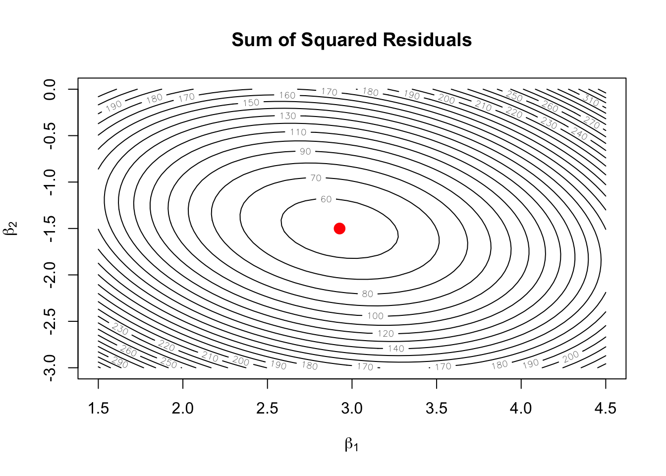
The contours are ellipses (because \(\mathbf{X}'\mathbf{X}\) is positive definite), and the red dot marks the OLS solution at the center.
9 The normal distribution
Many results in the course rely on normality, especially for small-sample inference. Here’s what different normal densities look like, and the key property that linear transformations preserve normality.
ggplot(data.frame(x = c(-5, 5)), aes(x)) +
  stat_function(fun = dnorm, args = list(mean = 0, sd = 1),
                aes(color = "N(0, 1)"), linewidth = 0.8) +
  stat_function(fun = dnorm, args = list(mean = 0, sd = sqrt(0.5)),
                aes(color = "N(0, 0.5)"), linewidth = 0.8) +
  stat_function(fun = dnorm, args = list(mean = 0, sd = sqrt(2)),
                aes(color = "N(0, 2)"), linewidth = 0.8) +
  scale_color_manual(values = c("steelblue", "tomato", "forestgreen"),
                     name = "") +
  labs(x = "x", y = "f(x)",
       title = "Normal densities with different variances") +
  theme_minimal()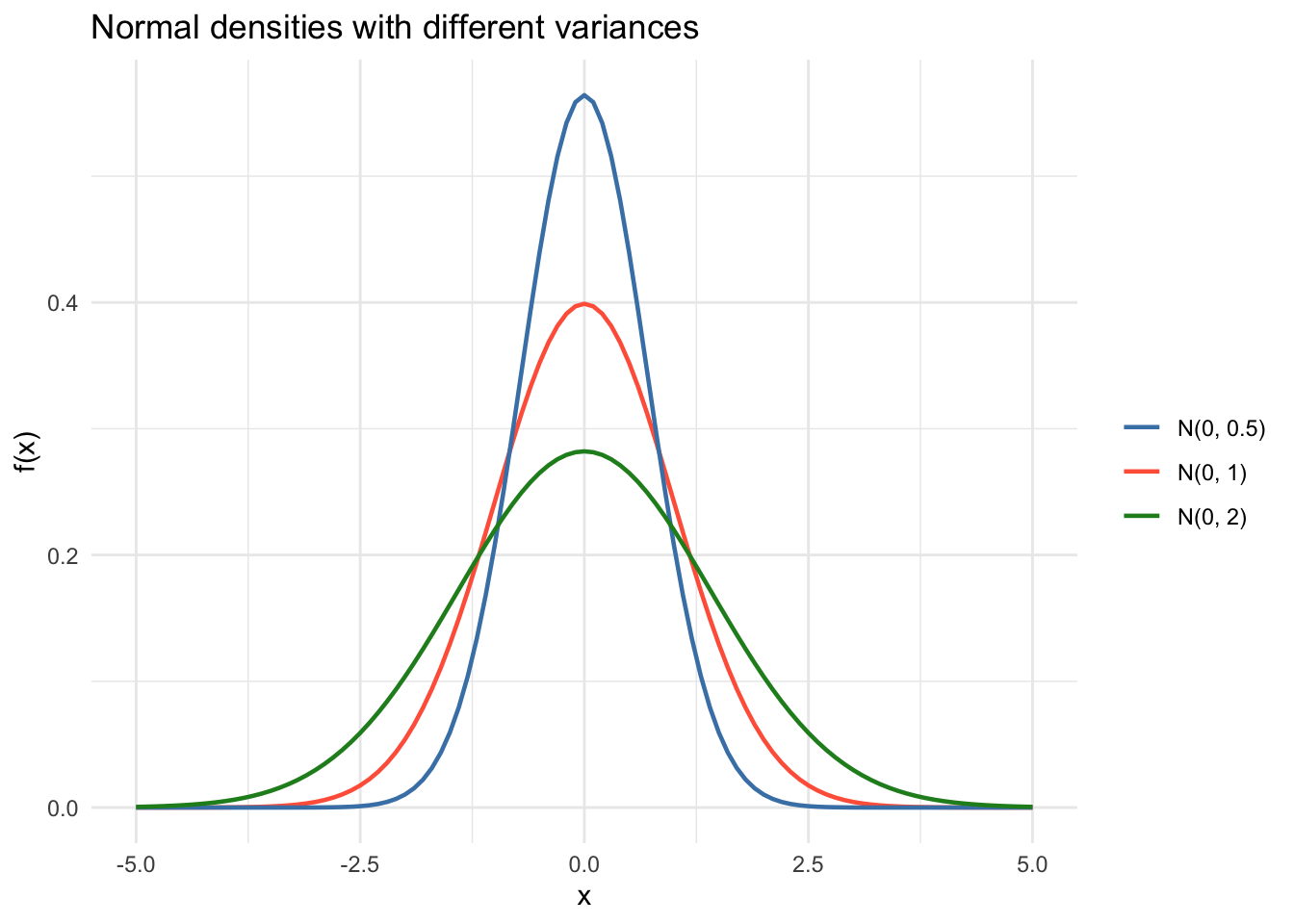
# If X ~ N(2, 3), then aX + b ~ N(a*2 + b, a^2 * 3)
set.seed(99)
X_samp <- rnorm(10000, mean = 2, sd = sqrt(3))
Y_samp <- 4 * X_samp + 1  # a = 4, b = 1

c(empirical_mean = mean(Y_samp), theoretical_mean = 4 * 2 + 1)
empirical_mean theoretical_mean
9.02 9.00 c(empirical_var = var(Y_samp), theoretical_var = 16 * 3) empirical_var theoretical_var
48.1 48.0 10 Summary
This chapter covered the computational foundations:
- Expectation minimizes mean squared error — the simplest prediction problem.
- The CEF generalizes this: the best prediction of \(Y\) given \(X\).
- The law of iterated expectations connects conditional and unconditional means.
- The law of total variance decomposes variance into explained and unexplained parts (\(R^2\)).
- The design matrix \(\mathbf{X}\) and Gram matrix \(\mathbf{X}'\mathbf{X}\) encode the regression problem.
- OLS is a projection of \(\mathbf{y}\) onto the column space of \(\mathbf{X}\).
- Positive definiteness guarantees a unique solution and a bowl-shaped objective.
- Degrees of freedom (\(n - k\)) come from the dimension of the residual space.
Next: The CEF and Best Linear Predictor — what happens when the CEF isn’t linear, and why linear regression still works.