library(ggplot2)
library(sandwich)
library(lmtest)
library(estimatr)
library(car)
library(carData)
options(digits = 4)

data(Salaries)9. Hypothesis Testing
The F-test, the test trinity, multiple testing, and power
Chapter 8 gave us sandwich standard errors and bootstrap confidence intervals. This chapter puts them to work: we test hypotheses, build confidence regions, guard against false discoveries, and ask whether our sample is large enough to detect effects we care about.
The emphasis is on doing — running tests in R, interpreting the output correctly, and avoiding common pitfalls. We organize around applied questions:
- How do I test whether a coefficient is zero? (t-tests, robust Wald)
- How do I test multiple restrictions at once? (F-test, joint Wald)
- Why Wald, not LR or classical F, is the default (the trinity under misspecification)
- How do I get confidence sets for nonlinear parameters? (test inversion, Fieller)
- What if I test many hypotheses? (Bonferroni, Holm)
- How large a sample do I need? (power analysis)
We use the Salaries dataset from carData throughout: salaries of 397 U.S. professors, with rank, discipline, years since PhD, years of service, and sex.
1 Testing a single coefficient
We start with a wage equation and ask: controlling for rank, discipline, and experience, does sex predict salary?
mod <- lm(salary ~ rank + discipline + yrs.since.phd + yrs.service + sex,
          data = Salaries)
summary(mod)
Call:
lm(formula = salary ~ rank + discipline + yrs.since.phd + yrs.service +
    sex, data = Salaries)

Residuals:
   Min     1Q Median     3Q    Max
-65248 -13211  -1775  10384  99592

Coefficients:
              Estimate Std. Error t value Pr(>|t|)
(Intercept)      65955       4589   14.37  < 2e-16 ***
rankAssocProf    12908       4145    3.11    0.002 **
rankProf         45066       4238   10.63  < 2e-16 ***
disciplineB      14418       2343    6.15  1.9e-09 ***
yrs.since.phd      535        241    2.22    0.027 *
yrs.service       -490        212   -2.31    0.021 *
sexMale           4784       3859    1.24    0.216
---
Signif. codes:  0 '***' 0.001 '**' 0.01 '*' 0.05 '.' 0.1 ' ' 1

Residual standard error: 22500 on 390 degrees of freedom
Multiple R-squared:  0.455, Adjusted R-squared:  0.446
F-statistic: 54.2 on 6 and 390 DF,  p-value: <2e-16
The summary() output gives t-statistics and p-values, but these assume homoskedasticity. The robust version uses sandwich standard errors:
coeftest(mod, vcov. = vcovHC(mod, type = "HC1"))
t test of coefficients:

              Estimate Std. Error t value Pr(>|t|)
(Intercept)      65955       2896   22.78  < 2e-16 ***
rankAssocProf    12908       2206    5.85  1.0e-08 ***
rankProf         45066       3285   13.72  < 2e-16 ***
disciplineB      14418       2316    6.22  1.2e-09 ***
yrs.since.phd      535        312    1.71    0.088 .
yrs.service       -490        307   -1.60    0.111
sexMale           4784       2396    2.00    0.047 *
---
Signif. codes:  0 '***' 0.001 '**' 0.01 '*' 0.05 '.' 0.1 ' ' 1
These are the same tests, built from the same Wald statistic \(W = (\hat{\beta}_j / \widehat{\text{se}}_j)^2\). The only difference is the denominator. When the two disagree, trust the robust version — it doesn’t assume \(\text{Var}(e_i \mid X_i)\) is constant.
You can also use linearHypothesis() for the same test, which makes the Wald structure explicit:
linearHypothesis(mod, "sexMale = 0", vcov. = vcovHC(mod, type = "HC1"))
Linear hypothesis test:
sexMale = 0

Model 1: restricted model
Model 2: salary ~ rank + discipline + yrs.since.phd + yrs.service + sex

Note: Coefficient covariance matrix supplied.

  Res.Df Df    F Pr(>F)
1    391
2    390  1 3.99  0.047 *
---
Signif. codes:  0 '***' 0.001 '**' 0.01 '*' 0.05 '.' 0.1 ' ' 1
This tests \(H_0: \beta_{\text{Male}} = 0\) against \(H_1: \beta_{\text{Male}} \neq 0\) using the robust covariance matrix. The Chisq column is the Wald statistic; divide by 1 (one restriction) and you get the squared t-statistic.
1.1 Testing against a non-zero value
Suppose theory predicts a gender gap of $5,000. The null is \(H_0: \beta_{\text{Male}} = 5000\):
linearHypothesis(mod, "sexMale = 5000", vcov. = vcovHC(mod, type = "HC1"))
Linear hypothesis test:
sexMale = 5000

Model 1: restricted model
Model 2: salary ~ rank + discipline + yrs.since.phd + yrs.service + sex

Note: Coefficient covariance matrix supplied.

  Res.Df Df    F Pr(>F)
1    391
2    390  1 0.01   0.93
The test is not significant if the confidence interval from Chapter 8 already contains $5,000. Test and CI carry exactly the same information — they are duals.
2 Testing multiple restrictions: the F-test
Individual t-tests tell you about one coefficient at a time. But sometimes you need a joint test. Does rank matter at all? That means testing two coefficients simultaneously (since rank is a three-level factor with two dummies):
\[H_0: \beta_{\text{AssocProf}} = \beta_{\text{Prof}} = 0\]
2.1 By hand: comparing two regressions
The F-test compares the fit of an unrestricted model to a restricted model that imposes \(H_0\):
\[F = \frac{(\text{SSE}_R - \text{SSE}_U) / q}{\text{SSE}_U / (n - k)}\]
where \(q\) is the number of restrictions.
## Unrestricted model (full)
mod_U <- mod

## Restricted model: drop rank
mod_R <- lm(salary ~ discipline + yrs.since.phd + yrs.service + sex,
            data = Salaries)

## Manual F-stat
SSE_U <- sum(resid(mod_U)^2)
SSE_R <- sum(resid(mod_R)^2)
q <- 2                              # two restrictions
n <- nobs(mod_U)
k <- length(coef(mod_U))

F_stat <- ((SSE_R - SSE_U) / q) / (SSE_U / (n - k))
p_val  <- 1 - pf(F_stat, q, n - k)

cat("F =", round(F_stat, 2), "  df1 =", q, "  df2 =", n - k,
    "  p =", format.pval(p_val), "\n")
F = 68.41 df1 = 2 df2 = 390 p = <2e-16 2.2 The easy way: anova() and linearHypothesis()
## Nested model comparison
anova(mod_R, mod_U)
Analysis of Variance Table
Model 1: salary ~ discipline + yrs.since.phd + yrs.service + sex
Model 2: salary ~ rank + discipline + yrs.since.phd + yrs.service + sex
Res.Df RSS Df Sum of Sq F Pr(>F)
1 392 2.68e+11
2 390 1.98e+11 2 6.95e+10 68.4 <2e-16 ***
---
Signif. codes: 0 '***' 0.001 '**' 0.01 '*' 0.05 '.' 0.1 ' ' 1## Same test via linearHypothesis (with robust SEs)
linearHypothesis(mod, c("rankAssocProf = 0", "rankProf = 0"),
vcov. = vcovHC(mod, type = "HC1"))
Linear hypothesis test:
rankAssocProf = 0
rankProf = 0

Model 1: restricted model
Model 2: salary ~ rank + discipline + yrs.since.phd + yrs.service + sex

Note: Coefficient covariance matrix supplied.

  Res.Df Df   F Pr(>F)
1    392
2    390  2 109 <2e-16 ***
---
Signif. codes:  0 '***' 0.001 '**' 0.01 '*' 0.05 '.' 0.1 ' ' 1
Note that anova() uses the classical (homoskedastic) F-test, while linearHypothesis() with a robust vcov. gives the heteroskedasticity-robust Wald test. In this example they agree; with strongly heteroskedastic data they might not.
2.3 Equality constraints
Does the return to years since PhD equal the return to years of service? This is \(H_0: \beta_{\text{yrs.phd}} = \beta_{\text{yrs.service}}\):
linearHypothesis(mod, "yrs.since.phd = yrs.service",
                 vcov. = vcovHC(mod, type = "HC1"))
Linear hypothesis test:
yrs.since.phd - yrs.service = 0

Model 1: restricted model
Model 2: salary ~ rank + discipline + yrs.since.phd + yrs.service + sex

Note: Coefficient covariance matrix supplied.

  Res.Df Df    F Pr(>F)
1    391
2    390  1 2.92  0.088 .
---
Signif. codes:  0 '***' 0.001 '**' 0.01 '*' 0.05 '.' 0.1 ' ' 1
This works because linearHypothesis() can test any linear restriction \(\mathbf{R}\boldsymbol{\beta} = \mathbf{r}\). Under the hood it constructs the restriction matrix \(\mathbf{R}\) and computes: \[W = (\mathbf{R}\hat{\boldsymbol{\beta}} - \mathbf{r})' [\mathbf{R}\hat{\mathbf{V}}\mathbf{R}']^{-1} (\mathbf{R}\hat{\boldsymbol{\beta}} - \mathbf{r}) \;\xrightarrow{d}\; \chi^2_q \tag{1}\]
Theorem 1 (Wald Statistic) For testing \(H_0: R\beta = r\), the Wald statistic is \(W = (R\hat\beta - r)'[R\hat{V}R']^{-1}(R\hat\beta - r) \xrightarrow{d} \chi^2_q\) under \(H_0\), where \(q\) is the number of restrictions. With robust \(\hat{V}\), the test is valid under heteroskedasticity.
3 The test trinity under misspecification
Three classical tests attack the same null \(H_0: R\beta = r\):
| Test | Based on | Needs to believe |
|---|---|---|
| Wald | distance from \(\hat\beta\) to the null | only the mean function (plus consistent \(\hat V\)) |
| Score / LM | slope of the objective at the restricted estimator | only the mean function (plus consistent “meat” matrix) |
| LR | height difference \(\log L_U - \log L_R\) | the full likelihood |
Two things about this table are worth dwelling on.
LR requires the likelihood. Under homoskedastic normal errors the classical F-test equals the LR statistic up to a monotone transformation, and the whole trinity is pedagogically unified. Once errors are heteroskedastic or the likelihood is otherwise misspecified, \(-2(\log L_R - \log L_U)\) no longer converges to \(\chi^2_q\) — it converges to a weighted sum of \(\chi^2_1\) random variables with unknown weights. There are Satterthwaite-style corrections (“quasi-LR”) but in practice applied econometrics has simply dropped LR as a default and uses Wald with sandwich variance. The same logic rules out the classical F from anova(), which is the homoskedastic LR for linear models.
Wald and Score have clean robust versions. Swap the classical variance for the sandwich: \[W = (R\hat\beta - r)'\,[R\,\hat V_{\text{HC}}\, R']^{-1}\,(R\hat\beta - r) \xrightarrow{d} \chi^2_q\] \[LM = \Big(\textstyle\sum s_i\Big)'\Big(\textstyle\sum s_i s_i'\Big)^{-1}\Big(\textstyle\sum s_i\Big) \xrightarrow{d} \chi^2_q\] The Wald is linearHypothesis(mod, ..., vcov = vcovHC(mod, type = "HC2")). The robust LM comes up most often not as a head-to-head rival to Wald but as the engine of specification tests — Breusch–Pagan for heteroskedasticity, White’s information-matrix test, and (Chapter 11) the GMM overidentification test are all score tests.
3.1 When do you still use the classical F?
One genuinely remaining niche: when you do believe errors are normal and homoskedastic, the classical F has an exact \(F_{q,\,n-K}\) distribution in finite samples, while the robust Wald is only asymptotic. At \(n = 20\) with trustworthy homoskedasticity, the classical F’s exact critical values can be better-calibrated than \(\chi^2_q\). By \(n = 200\) this advantage vanishes.
3.2 A concrete comparison
## Joint test: rank has no effect (q = 2 restrictions)
## Classical F (homoskedastic)
anova(mod_R, mod_U)$F[2]
[1] 68.41## Robust Wald (heteroskedasticity-robust)
linearHypothesis(mod_U, c("rankAssocProf = 0", "rankProf = 0"),
vcov = vcovHC(mod_U, type = "HC2"),
test = "F")$F[2][1] 108.7The two statistics answer slightly different questions: classical F asks “under the homoskedastic-normal model, does fit deteriorate?”; robust Wald asks “given the estimated sandwich covariance, is \(R\hat\beta\) far from \(r\)?” When errors are actually homoskedastic they give nearly identical numbers. Otherwise, trust the robust version.
3.3 Where Score tests live
Score tests show up throughout the course, mostly not labeled as such:
- Breusch–Pagan (ch05): score test against \(H_0: \text{Var}(e_i \mid X_i)\) = constant.
- RESET (ch04): score test against \(H_0:\) no omitted nonlinear terms.
- Hausman (ch12): comparison of two estimators is equivalent to a score-type test.
- GMM overidentification / \(J\)-test (ch11): the canonical modern score test — are extra moment conditions satisfied at the efficient estimator?
The common thread: score tests only require the null fit. You estimate under \(H_0\) and ask whether the remaining moment conditions or specification implications are satisfied at that estimate. Two reasons this is the right tool:
- There may be no alternative model to fit. In GMM overidentification you have more moment conditions than parameters. There is no larger model that uses them all as free structure — the extras are just claims about the true \(\theta\). The score test asks: at the estimate pinned down by \(K\) moments, are the remaining \(L - K\) moments close to zero?
- The alternative is too broad to parametrize. Breusch–Pagan tests against “some form of heteroskedasticity” without naming which form. You don’t want to fit every possible heteroskedastic model; you want to check whether the residuals from the homoskedastic fit betray any systematic pattern.
In both cases, Wald is not available — there is nothing unrestricted to compare against. The score test is what you reach for.
4 Confidence regions and test inversion
A 95% confidence interval is the set of values \(\theta_0\) that would not be rejected at the 5% level:
\[\hat{C} = \{\theta_0 : |T(\theta_0)| \leq 1.96\}\]
This is test inversion. For a single linear coefficient, test inversion gives the familiar \(\hat{\beta} \pm 1.96 \cdot \widehat{\text{se}}\). But for nonlinear functions of parameters, test inversion is more reliable than the delta method.
NoteTest Inversion Gives Confidence Sets
A 95% confidence set is exactly the set of parameter values not rejected at the 5% level. For linear parameters, this gives the familiar \(\hat\beta \pm 1.96 \cdot \text{SE}\). For nonlinear functions, Fieller’s method (test inversion over a grid) is more reliable than the delta method.
4.1 Confidence ellipses for two coefficients
For two parameters tested jointly, the confidence region is an ellipse — the set of \((\beta_1, \beta_2)\) values consistent with the Wald test:
## Joint confidence region for the two experience variables
confidenceEllipse(mod, which.coef = c("yrs.since.phd", "yrs.service"),
                  vcov. = vcovHC(mod, type = "HC1"),
                  main = "95% joint confidence region",
                  xlab = "Coefficient on yrs.since.phd",
                  ylab = "Coefficient on yrs.service",
                  col = "steelblue", lwd = 2)
abline(h = 0, lty = 2, col = "gray50")
abline(v = 0, lty = 2, col = "gray50")
## Add the 45-degree line for equality
abline(a = 0, b = 1, lty = 3, col = "coral", lwd = 1.5)
legend("topright", legend = c("95% joint region", "equality line"),
       col = c("steelblue", "coral"), lty = c(1, 3), lwd = c(2, 1.5))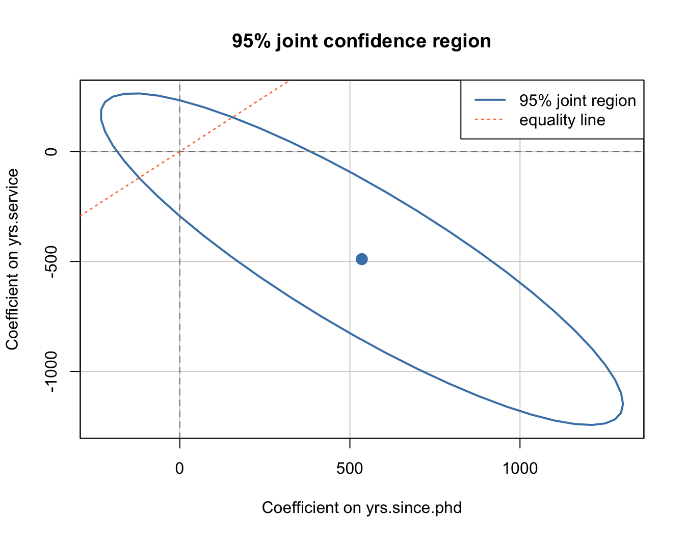
The dashed lines at zero show the individual null values. The coral line shows where the two coefficients are equal. If the ellipse crosses a line, the corresponding null cannot be rejected.
4.2 Test inversion for a nonlinear parameter: Fieller’s method
Suppose we want a confidence interval for the ratio \(\theta = \beta_{\text{Prof}} / \beta_{\text{AssocProf}}\) — how many times larger is the full professor salary premium than the associate professor premium? The delta method (Chapter 8) gives a quick CI, but it can be unreliable when the denominator is imprecisely estimated.
Fieller’s trick: rewrite \(\theta = \beta_1 / \beta_2\) as the linear restriction \(\beta_1 - \theta \beta_2 = 0\), then invert the Wald test over a grid of \(\theta\) values:
b <- coef(mod)
V <- vcovHC(mod, type = "HC1")

## Delta method CI for comparison
dm <- deltaMethod(mod, "rankProf / rankAssocProf",
                  vcov. = vcovHC(mod, type = "HC1"))
dm_ci <- c(dm$Estimate - 1.96 * dm$SE, dm$Estimate + 1.96 * dm$SE)

## Grid search: invert the Wald test
theta_grid <- seq(0, 8, by = 0.01)
idx_prof <- which(names(b) == "rankProf")
idx_assoc <- which(names(b) == "rankAssocProf")

in_CI <- sapply(theta_grid, function(th) {
  r_vec <- numeric(length(b))
  r_vec[idx_prof] <- 1
  r_vec[idx_assoc] <- -th
  num <- (sum(r_vec * b))^2
  den <- t(r_vec) %*% V %*% r_vec
  num / den <= qchisq(0.95, 1)
})
fieller_ci <- range(theta_grid[in_CI])

cat("Point estimate:  ", round(dm$Estimate, 3), "\n")
Point estimate: 3.491 cat("Delta method CI: ", round(dm_ci, 3), "\n")Delta method CI: 2.602 4.381 cat("Fieller CI: ", round(fieller_ci, 3), "\n")Fieller CI: 2.81 4.79 Here the two CIs are similar because the denominator (\(\beta_{\text{AssocProf}}\)) is precisely estimated. The ratio tells us that the full professor premium is about 3.5 times the associate professor premium.
## Plot the Wald statistic over theta
wald_vals <- sapply(theta_grid, function(th) {
  r_vec <- numeric(length(b))
  r_vec[idx_prof] <- 1
  r_vec[idx_assoc] <- -th
  num <- (sum(r_vec * b))^2
  den <- c(t(r_vec) %*% V %*% r_vec)
  num / den
})

df_fieller <- data.frame(theta = theta_grid, W = wald_vals)
ggplot(df_fieller, aes(theta, W)) +
  geom_line(color = "steelblue", linewidth = 0.8) +
  geom_hline(yintercept = qchisq(0.95, 1), linetype = "dashed", color = "coral") +
  annotate("text", x = 6.5, y = qchisq(0.95, 1) + 0.5, label = "95% critical value",
           color = "coral") +
  coord_cartesian(ylim = c(0, 15)) +
  labs(title = "Test inversion: Wald statistic as a function of θ₀",
       subtitle = "The Fieller CI is the set of θ₀ values below the dashed line",
       x = expression(theta[0] == beta[Prof] / beta[AssocProf]),
       y = "Wald statistic")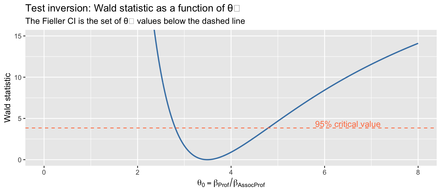
4.3 When Fieller and the delta method disagree
The real value of Fieller’s method appears when the denominator is imprecise. Consider \(\theta = \beta_{\text{yrs.phd}} / \beta_{\text{yrs.service}}\) — the ratio of the two experience coefficients. Both are individually insignificant:
## Experience coefficients are imprecise
cat("yrs.since.phd: estimate =", round(b["yrs.since.phd"]),
    "  SE =", round(sqrt(V["yrs.since.phd", "yrs.since.phd"])), "\n")
yrs.since.phd: estimate = 535 SE = 312 cat("yrs.service: estimate =", round(b["yrs.service"]),
" SE =", round(sqrt(V["yrs.service", "yrs.service"])), "\n")yrs.service: estimate = -490 SE = 307 ## Delta method gives a finite CI
dm2 <- deltaMethod(mod, "yrs.since.phd / yrs.service",
vcov. = vcovHC(mod, type = "HC1"))
cat("\nDelta method CI:", round(c(dm2$Estimate - 1.96 * dm2$SE,
dm2$Estimate + 1.96 * dm2$SE), 2), "\n")
Delta method CI: -1.75 -0.43 ## Fieller: check a wide grid
theta_wide <- seq(-50, 50, by = 0.1)
idx_phd <- which(names(b) == "yrs.since.phd")
idx_svc <- which(names(b) == "yrs.service")
in_CI2 <- sapply(theta_wide, function(th) {
r_vec <- numeric(length(b))
r_vec[idx_phd] <- 1
r_vec[idx_svc] <- -th
num <- (sum(r_vec * b))^2
den <- c(t(r_vec) %*% V %*% r_vec)
num / den <= qchisq(0.95, 1)
})
## Check if CI covers entire grid (unbounded)
if (all(in_CI2)) {
cat("Fieller CI: (-∞, +∞) [unbounded!]\n")
} else if (any(in_CI2)) {
cat("Fieller CI:", range(theta_wide[in_CI2]), "\n")
}Fieller CI: (-∞, +∞) [unbounded!]The delta method reports a finite CI of width ~1.3, but the Fieller CI is unbounded — the entire real line. This is the correct answer: since \(\beta_{\text{yrs.service}}\) is not significantly different from zero, the ratio could be anything. The delta method’s finite interval is overconfident.
5 Multiple testing
When you look at many coefficients, some will be “significant” by chance.
5.1 Simulation: false discoveries under the null
To make this concrete: generate 20 pure-noise regressors, test each at 5%, and count how many reject:
set.seed(303)
n <- 200
k_noise <- 20
Y <- rnorm(n)
X_noise <- matrix(rnorm(n * k_noise), nrow = n)
colnames(X_noise) <- paste0("X", 1:k_noise)
dat_noise <- data.frame(Y, X_noise)

mod_noise <- lm(Y ~ ., data = dat_noise)
pvals <- summary(mod_noise)$coefficients[-1, 4]  # drop intercept

cat("Number of regressors with p < 0.05:", sum(pvals < 0.05), "out of", k_noise, "\n")
Number of regressors with p < 0.05: 1 out of 20 cat("Significant variables:", paste(names(pvals[pvals < 0.05]), collapse = ", "), "\n")Significant variables: X12 Under the global null, we expect \(20 \times 0.05 = 1\) false rejection on average. Repeat this many times to see the problem clearly:
set.seed(42)
B <- 5000
n <- 200
k_noise <- 20

false_rejections <- replicate(B, {
  Y <- rnorm(n)
  X <- matrix(rnorm(n * k_noise), nrow = n)
  pv <- summary(lm(Y ~ X))$coefficients[-1, 4]
  sum(pv < 0.05)
})

cat("P(at least one false rejection):", mean(false_rejections >= 1), "\n")
P(at least one false rejection): 0.6204 cat("Expected:", round(1 - (1 - 0.05)^k_noise, 3), "\n")Expected: 0.642 ggplot(data.frame(rejections = false_rejections), aes(rejections)) +
geom_bar(fill = "steelblue", alpha = 0.7) +
geom_vline(xintercept = 1, linetype = "dashed", color = "coral") +
labs(title = "False rejections when all 20 nulls are true",
subtitle = paste0("P(≥1 false rejection) = ",
round(mean(false_rejections >= 1), 3)),
x = "Number of rejections at α = 0.05",
y = "Frequency")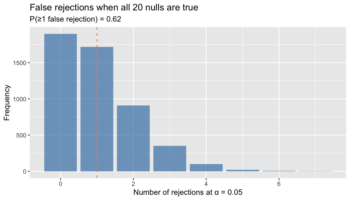
With 20 tests at 5%, you have about a 64% chance of at least one false rejection. This is the familywise error rate (FWER) problem.
WarningMultiple Testing Inflates the Familywise Error Rate
With \(k\) independent tests at level \(\alpha\), the probability of at least one false rejection is \(1 - (1 - \alpha)^k\). With 20 tests at 5%, this exceeds 60%. Use Holm’s correction (uniformly more powerful than Bonferroni) to control the FWER.
5.2 Corrections: Bonferroni and Holm
The Bonferroni correction rejects the \(j\)th hypothesis only if \(p_j < \alpha / k\). It controls the FWER for any dependence structure:
## Back to our salary model
pvals_salary <- summary(mod)$coefficients[-1, 4]

corrections <- data.frame(
  raw = round(pvals_salary, 4),
  bonferroni = round(p.adjust(pvals_salary, method = "bonferroni"), 4),
  holm = round(p.adjust(pvals_salary, method = "holm"), 4)
)
corrections
raw bonferroni holm
rankAssocProf 0.0020 0.0119 0.0079
rankProf 0.0000 0.0000 0.0000
disciplineB 0.0000 0.0000 0.0000
yrs.since.phd 0.0270 0.1619 0.0643
yrs.service 0.0214 0.1286 0.0643
sexMale 0.2158 1.0000 0.2158Holm’s method is uniformly more powerful than Bonferroni while still controlling the FWER. It works by ordering the p-values from smallest to largest and comparing the \(j\)th smallest to \(\alpha / (k - j + 1)\). Use Holm whenever you would use Bonferroni.
5.3 When to worry about multiple testing
Multiple testing corrections matter when you:
- Examine many coefficients and report the “most significant”
- Try many specifications and present the one that “works”
- Test across subgroups (by age, gender, region, …)
- Use stepwise selection procedures
They matter less when you have a small number of pre-specified hypotheses motivated by theory.
6 Power: can you detect the effect?
A test’s power is the probability it rejects when \(H_0\) is false:
\[\text{Power}(\theta) = P[\text{Reject } H_0 \mid \theta \neq \theta_0]\]
Power depends on four things: the true effect size, the standard error, the significance level, and the sample size. In OLS, for a two-sided test of \(H_0: \beta = 0\):
\[\delta = \frac{|\beta|}{\text{se}(\hat{\beta})} \approx \frac{|\beta| \cdot \text{sd}(X) \cdot \sqrt{n}}{\sigma_e}\]
Power \(\approx \Phi(\delta - z_{\alpha/2}) + \Phi(-\delta - z_{\alpha/2})\), where \(\delta\) is the signal-to-noise ratio.
Theorem 2 (Power of a Two-Sided Test) For testing \(H_0: \beta = 0\) at level \(\alpha\), the power against alternative \(\beta \neq 0\) is approximately \(\Phi(\delta - z_{\alpha/2}) + \Phi(-\delta - z_{\alpha/2})\), where \(\delta = |\beta|/\text{SE}(\hat\beta)\) is the signal-to-noise ratio.
## Power for a two-sided t-test in OLS
power_ols <- function(effect, sigma_e, sd_x, n, alpha = 0.05) {
  se <- sigma_e / (sd_x * sqrt(n))
  delta <- abs(effect) / se
  z <- qnorm(1 - alpha / 2)
  pnorm(delta - z) + pnorm(-delta - z)
}
6.1 Power curves
How does power vary with sample size and effect size?
n_seq <- seq(20, 500, by = 5)
effects <- c(0.05, 0.10, 0.20, 0.40)

df_power <- do.call(rbind, lapply(effects, function(eff) {
  data.frame(
    n = n_seq,
    power = sapply(n_seq, function(nn) power_ols(eff, sigma_e = 1, sd_x = 1, nn)),
    effect = paste0("β = ", eff)
  )
}))

ggplot(df_power, aes(n, power, color = effect)) +
  geom_line(linewidth = 1) +
  geom_hline(yintercept = 0.80, linetype = "dashed", color = "gray50") +
  annotate("text", x = 480, y = 0.82, label = "80% power", color = "gray50") +
  geom_hline(yintercept = 0.05, linetype = "dotted", color = "gray70") +
  annotate("text", x = 480, y = 0.07, label = "α = 0.05", color = "gray70") +
  scale_color_brewer(palette = "Set1") +
  labs(title = "Power curves for a two-sided OLS t-test",
       subtitle = "σ_e = 1, sd(X) = 1",
       x = "Sample size (n)", y = "Power", color = "True effect") +
  coord_cartesian(ylim = c(0, 1))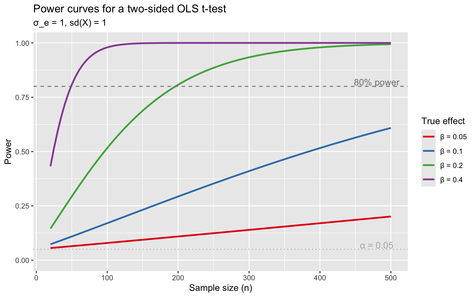
Small effects require enormous samples. With \(\beta = 0.10\) and \(\sigma_e / \text{sd}(X) = 1\), you need roughly \(n = 800\) for 80% power.
TipThe 80% Power Rule of Thumb
A study should have at least 80% power to detect the smallest effect of scientific interest. This requires \(n \approx 16\sigma_e^2 / (\beta^2 \cdot \text{Var}(X))\) for a two-sided 5% test. Adding relevant controls reduces \(\sigma_e\) and boosts power for free.
6.2 Simulation: observing power
Let’s verify the formula with a Monte Carlo simulation:
set.seed(12)
B <- 2000
true_beta <- 0.3
sigma_e <- 1
n_vals <- c(20, 50, 100, 200)

sim_power <- function(n, B) {
  rejections <- replicate(B, {
    x <- rnorm(n)
    y <- true_beta * x + rnorm(n, sd = sigma_e)
    pval <- summary(lm(y ~ x))$coefficients["x", "Pr(>|t|)"]
    pval < 0.05
  })
  mean(rejections)
}

results <- data.frame(
  n = n_vals,
  simulated = sapply(n_vals, sim_power, B = B),
  formula = sapply(n_vals, function(nn) power_ols(true_beta, sigma_e, 1, nn))
)
results
n simulated formula
1 20 0.2290 0.2687
2 50 0.5575 0.5641
3 100 0.8250 0.8508
4 200 0.9880 0.9888The simulated power matches the formula closely.
6.3 Controls boost power
Adding a relevant control variable reduces \(\sigma_e\) without reducing \(\text{sd}(X)\), giving a free power boost:
set.seed(99)
B <- 2000
n <- 100
beta_x <- 0.2
beta_z <- 1.0  # strong control

## Without control
power_no_ctrl <- mean(replicate(B, {
  x <- rnorm(n); z <- rnorm(n)
  y <- beta_x * x + beta_z * z + rnorm(n)
  summary(lm(y ~ x))$coefficients["x", "Pr(>|t|)"] < 0.05
}))

## With control
power_with_ctrl <- mean(replicate(B, {
  x <- rnorm(n); z <- rnorm(n)
  y <- beta_x * x + beta_z * z + rnorm(n)
  summary(lm(y ~ x + z))$coefficients["x", "Pr(>|t|)"] < 0.05
}))

cat("Power without control:", round(power_no_ctrl, 3), "\n")
Power without control: 0.294 cat("Power with control: ", round(power_with_ctrl, 3), "\n")Power with control: 0.5 cat("Residual SD without z:", round(sqrt(beta_z^2 + 1), 2), "\n")Residual SD without z: 1.41 cat("Residual SD with z: ", round(1, 2), "\n")Residual SD with z: 1 The control cuts the residual standard deviation roughly in half, dramatically increasing power. This is why pre-treatment covariates help in experiments even though they are unnecessary for unbiasedness.
6.4 Joint tests have less power
Testing more restrictions simultaneously dilutes power. Fix the total non-centrality parameter and compare:
lambda_seq <- seq(0, 15, by = 0.1)

df_joint <- do.call(rbind, lapply(c(1, 2, 5, 10), function(q) {
  data.frame(
    lambda = lambda_seq,
    power = 1 - pchisq(qchisq(0.95, q), q, ncp = lambda_seq),
    q = paste0("q = ", q)
  )
}))

ggplot(df_joint, aes(lambda, power, color = q)) +
  geom_line(linewidth = 1) +
  geom_hline(yintercept = 0.80, linetype = "dashed", color = "gray50") +
  scale_color_brewer(palette = "Set1") +
  labs(title = "Power vs. non-centrality for joint tests",
       subtitle = "More restrictions require a larger signal to achieve the same power",
       x = expression(paste("Non-centrality parameter ", lambda)),
       y = "Power", color = "Restrictions")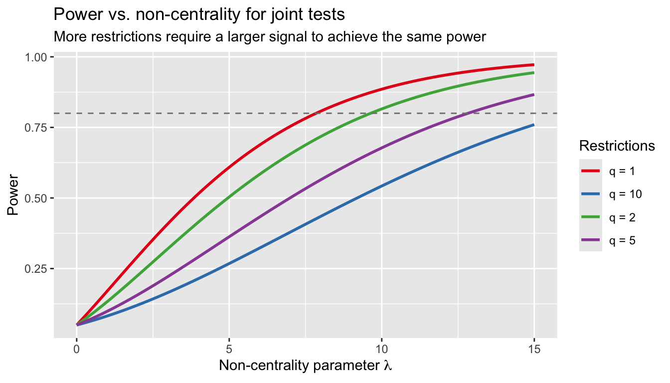
A single-coefficient t-test is more powerful than a joint F-test that lumps in other restrictions. Test exactly what you care about.
7 Statistical vs. economic significance
With a large enough sample, any nonzero coefficient becomes statistically significant. This is test consistency: \(P[\text{Reject}] \to 1\) whenever \(\beta \neq 0\).
set.seed(77)
true_beta <- 0.01   # tiny effect
n_vals <- c(50, 200, 1000, 5000, 20000)
B <- 1000

rejection_rate <- sapply(n_vals, function(nn) {
  mean(replicate(B, {
    x <- rnorm(nn)
    y <- true_beta * x + rnorm(nn)
    summary(lm(y ~ x))$coefficients["x", "Pr(>|t|)"] < 0.05
  }))
})

df_consist <- data.frame(n = n_vals, rejection_rate = rejection_rate)
ggplot(df_consist, aes(n, rejection_rate)) +
  geom_line(linewidth = 1, color = "steelblue") +
  geom_point(size = 3, color = "steelblue") +
  geom_hline(yintercept = 0.05, linetype = "dashed", color = "coral") +
  scale_x_log10() +
  labs(title = "Test consistency: even β = 0.01 gets rejected eventually",
       subtitle = "With enough data, statistical significance is guaranteed for any nonzero effect",
       x = "Sample size (log scale)", y = "Rejection rate at α = 0.05")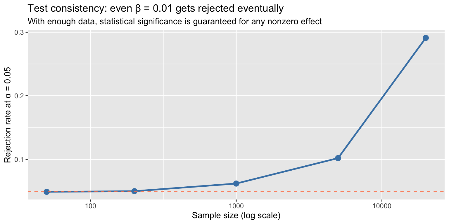
A \(p\)-value tells you whether the data are inconsistent with \(H_0\). It tells you nothing about whether the effect is large enough to matter. Always report the magnitude alongside the significance.
8 Applied workflow: the salary example
Let’s bring everything together with a thorough analysis of the professor salary data.
8.1 Step 1: Fit and inspect
mod_full <- lm(salary ~ rank + discipline + yrs.since.phd + yrs.service + sex,
               data = Salaries)
coeftest(mod_full, vcov. = vcovHC(mod_full, type = "HC1"))
t test of coefficients:

              Estimate Std. Error t value Pr(>|t|)
(Intercept)      65955       2896   22.78  < 2e-16 ***
rankAssocProf    12908       2206    5.85  1.0e-08 ***
rankProf         45066       3285   13.72  < 2e-16 ***
disciplineB      14418       2316    6.22  1.2e-09 ***
yrs.since.phd      535        312    1.71    0.088 .
yrs.service       -490        307   -1.60    0.111
sexMale           4784       2396    2.00    0.047 *
---
Signif. codes:  0 '***' 0.001 '**' 0.01 '*' 0.05 '.' 0.1 ' ' 1
8.2 Step 2: Key hypotheses
Does rank matter? (joint test, \(q = 2\))
linearHypothesis(mod_full, c("rankAssocProf = 0", "rankProf = 0"),
                 vcov. = vcovHC(mod_full, type = "HC1"))
Linear hypothesis test:
rankAssocProf = 0
rankProf = 0

Model 1: restricted model
Model 2: salary ~ rank + discipline + yrs.since.phd + yrs.service + sex

Note: Coefficient covariance matrix supplied.

  Res.Df Df   F Pr(>F)
1    392
2    390  2 109 <2e-16 ***
---
Signif. codes:  0 '***' 0.001 '**' 0.01 '*' 0.05 '.' 0.1 ' ' 1
Does discipline matter? (single restriction)
linearHypothesis(mod_full, "disciplineB = 0",
                 vcov. = vcovHC(mod_full, type = "HC1"))
Linear hypothesis test:
disciplineB = 0

Model 1: restricted model
Model 2: salary ~ rank + discipline + yrs.since.phd + yrs.service + sex

Note: Coefficient covariance matrix supplied.

  Res.Df Df    F  Pr(>F)
1    391
2    390  1 38.7 1.2e-09 ***
---
Signif. codes:  0 '***' 0.001 '**' 0.01 '*' 0.05 '.' 0.1 ' ' 1
Are the two experience measures interchangeable? (\(\beta_{\text{phd}} = \beta_{\text{svc}}\))
linearHypothesis(mod_full, "yrs.since.phd = yrs.service",
                 vcov. = vcovHC(mod_full, type = "HC1"))
Linear hypothesis test:
yrs.since.phd - yrs.service = 0

Model 1: restricted model
Model 2: salary ~ rank + discipline + yrs.since.phd + yrs.service + sex

Note: Coefficient covariance matrix supplied.

  Res.Df Df    F Pr(>F)
1    391
2    390  1 2.92  0.088 .
---
Signif. codes:  0 '***' 0.001 '**' 0.01 '*' 0.05 '.' 0.1 ' ' 1
8.3 Step 3: Confidence intervals
## Robust CIs
ci_robust <- coefci(mod_full, vcov. = vcovHC(mod_full, type = "HC1"))
ci_robust
2.5 % 97.5 %
(Intercept) 60261.83 71648.6
rankAssocProf 8571.09 17244.1
rankProf 38607.31 51524.7
disciplineB 9863.61 18971.6
yrs.since.phd -79.26 1149.4
yrs.service -1092.74 113.7
sexMale 72.96 9494.08.4 Step 4: Multiple testing adjustment
If we’re testing all six regressors simultaneously:
pvals_all <- coeftest(mod_full, vcov. = vcovHC(mod_full, type = "HC1"))[-1, 4]
data.frame(
  raw_p = round(pvals_all, 4),
  holm_p = round(p.adjust(pvals_all, method = "holm"), 4),
  significant_raw = ifelse(pvals_all < 0.05, "*", ""),
  significant_holm = ifelse(p.adjust(pvals_all, method = "holm") < 0.05, "*", "")
)
raw_p holm_p significant_raw significant_holm
rankAssocProf 0.0000 0.0000 * *
rankProf 0.0000 0.0000 * *
disciplineB 0.0000 0.0000 * *
yrs.since.phd 0.0876 0.1752
yrs.service 0.1114 0.1752
sexMale 0.0466 0.1397 * 8.5 Step 5: Power assessment for the gender gap
Suppose the “true” gender gap is $5,000 (about 5% of mean salary). Could we detect it?
sigma_e <- sigma(mod_full)
sd_sex <- sd(as.numeric(Salaries$sex == "Male"))
n <- nrow(Salaries)

power_sex <- power_ols(effect = 5000, sigma_e = sigma_e,
                       sd_x = sd_sex, n = n, alpha = 0.05)
cat("Estimated power to detect a $5,000 gender gap:", round(power_sex, 3), "\n")
Estimated power to detect a $5,000 gender gap: 0.261 ## What sample size for 80% power?
n_needed <- seq(100, 5000, by = 10)
pow_curve <- sapply(n_needed, function(nn)
power_ols(5000, sigma_e, sd_sex, nn, 0.05))
n80 <- n_needed[which(pow_curve >= 0.80)[1]]
cat("Sample size for 80% power:", n80, "\n")Sample size for 80% power: 1800 9 Practical advice (after Hansen)
A checklist for reporting regression results:
Report standard errors, not just t-ratios. Standard errors convey precision; t-statistics reduce everything to a binary yes/no.
Report p-values, not asterisks. The difference between \(p = 0.049\) and \(p = 0.051\) is not meaningful. Stars obscure this.
Focus on substantive hypotheses. Don’t mechanically test every coefficient against zero. Test things that answer a scientific question.
“Fail to reject” \(\neq\) “accept.” Low power can explain non-rejection. Always ask: could we have detected a meaningful effect?
Statistical significance \(\neq\) economic significance. A tiny but significant coefficient may be policy-irrelevant. A large but insignificant coefficient may reflect low power.
Use robust inference by default. There is rarely a good reason to report classical SEs when \(n\) is not tiny. Use HC1/HC2 or the bootstrap.
Account for multiple testing. If you report the “most significant” result from many tests, apply Holm or Bonferroni corrections.
10 Connection to GMM
The Wald test has a natural GMM interpretation. In GMM, testing \(H_0: \mathbf{R}\boldsymbol{\beta} = \mathbf{r}\) is equivalent to testing whether the restricted moment conditions \(E[\mathbf{Z}'(Y - \mathbf{X}\boldsymbol{\beta})] = \mathbf{0}\) with \(\mathbf{R}\boldsymbol{\beta} = \mathbf{r}\) are compatible with the data. The J-test of overidentifying restrictions, which we’ll meet in Chapter 11, generalizes the F-test to the setting where there are more moment conditions than parameters.
| OLS test | GMM counterpart |
|---|---|
| F-test (restricted vs. unrestricted) | Distance test (restricted vs. unrestricted GMM) |
| Wald test | Wald test (same formula, different \(\hat{\mathbf{V}}\)) |
| Score / LM test | Score test from restricted GMM |
| Overall F-statistic | J-test of overidentifying restrictions |