6. Small Sample Inference

Likelihood, the normal linear model, and exact tests

The previous chapters derived the OLS estimator using only moment conditions — no distributional assumptions required. This chapter adds the assumption that errors are normal, which unlocks exact finite-sample distributions for $\hat{\beta}$, $s^2$, and the $t$- and $F$-statistics. We build everything computationally: write the likelihood, verify MLE = OLS, simulate the distributional results, and apply them to real data.

Questions this chapter answers:

How does the likelihood function connect to OLS, and why does MLE give the same $\hat\beta$?
What exact sampling distributions do $\hat\beta$, $s^2$, and the $t$-statistic follow under normality?
How do we conduct applied inference — $t$-tests, $F$-tests, and confidence intervals — in R?
When do exact tests break down, and what alternatives exist?

library(ggplot2)
library(sandwich)
library(lmtest)
library(estimatr)
library(car)
options(digits = 3)

1 Likelihood

A parametric model specifies a probability density $f(x \mid \theta)$ for the data. The likelihood reverses the role of data and parameters: given observed data, how probable is each parameter value?

1.1 Example: binomial likelihood

Suppose we observe the number of terms served by 5 legislators: $x = \{1, 0, 1, 2, 0\}$, each out of 2 possible terms. The binomial probability is $P(x_i \mid p) = \binom{2}{x_i} p^{x_i}(1-p)^{2-x_i}$.

x_obs <- c(1, 0, 1, 2, 0)
n_trials <- 2

# Likelihood as a function of p
lik <- function(p) {
  prod(dbinom(x_obs, size = n_trials, prob = p))
}

p_grid <- seq(0.01, 0.99, by = 0.01)
lik_vals <- sapply(p_grid, lik)

df_lik <- data.frame(p = p_grid, likelihood = lik_vals)
ggplot(df_lik, aes(p, likelihood)) +
  geom_line(linewidth = 1) +
  geom_vline(xintercept = p_grid[which.max(lik_vals)], linetype = "dashed", color = "red") +
  labs(title = "Binomial likelihood for x = {1, 0, 1, 2, 0}",
       subtitle = paste("MLE: p̂ =", p_grid[which.max(lik_vals)]),
       x = "p", y = "L(p | x)")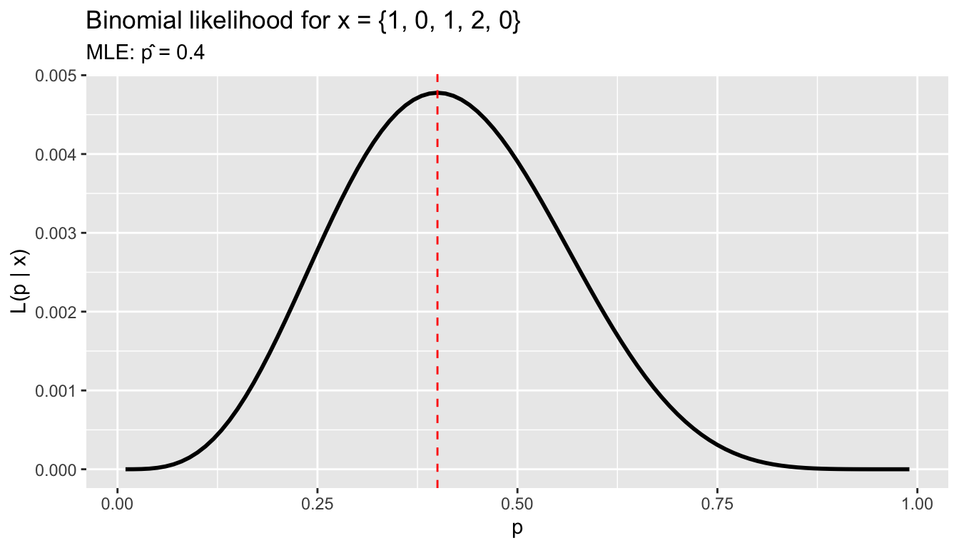

The MLE is $\hat{p} = \sum x_i / (n \cdot 2) = 4/10 = 0.4$ — the sample proportion.

1.2 The log-likelihood

We almost always work with the log-likelihood $\ell(\theta) = \sum \log f(x_i \mid \theta)$, which turns products into sums and is easier to optimize:

loglik <- function(p) sum(dbinom(x_obs, size = n_trials, prob = p, log = TRUE))

# Optimize
opt <- optimize(loglik, interval = c(0, 1), maximum = TRUE)
opt$maximum

[1] 0.4

1.3 Score, Hessian, and Fisher information

The score is the derivative of the log-likelihood — it tells you the slope at any parameter value. At the MLE, the score equals zero:

# Score for binomial: d/dp [sum(x*log(p) + (2-x)*log(1-p))]
# = sum(x)/p - sum(2-x)/(1-p)
score <- function(p) sum(x_obs) / p - sum(n_trials - x_obs) / (1 - p)
score(0.4)  # zero at the MLE

[1] 0

# Hessian (negative second derivative): observed information
hessian <- function(p) sum(x_obs) / p^2 + sum(n_trials - x_obs) / (1 - p)^2
observed_info <- hessian(0.4)

# Cramér-Rao bound: variance >= 1 / information
c(observed_information = observed_info,
  CR_bound_variance    = 1 / observed_info,
  CR_bound_se          = 1 / sqrt(observed_info))

observed_information    CR_bound_variance          CR_bound_se 
              41.667                0.024                0.155

The Fisher information measures how sharply the likelihood peaks — more information means more precise estimation.

2 The normal linear model

The classic normal regression model adds a distributional assumption to OLS:

\[y \mid X \sim N(X\beta, \, \sigma^2 I)\]

This gives us the likelihood:

\[\mathcal{L}(\beta, \sigma^2) = (2\pi\sigma^2)^{-n/2} \exp\!\left(-\frac{1}{2\sigma^2} \sum_{i=1}^n (y_i - x_i'\beta)^2\right) \tag{1}\]

2.1 Writing the log-likelihood in R

data(swiss)
y <- swiss$Fertility
X <- model.matrix(~ Education + Agriculture + Catholic + Infant.Mortality,
                  data = swiss)
n <- nrow(X)
K <- ncol(X)

# Log-likelihood as a function of beta and sigma^2
normal_loglik <- function(beta, sigma2) {
  resid <- y - X %*% beta
  -n/2 * log(2 * pi * sigma2) - sum(resid^2) / (2 * sigma2)
}

2.2 MLE = OLS

Maximizing the normal log-likelihood with respect to $\beta$ gives $\hat{\beta}_{MLE} = (X'X)^{-1}X'y$ — exactly OLS. For $\sigma^2$, the MLE is $\hat{\sigma}^2_{MLE} = \frac{1}{n}\sum \hat{e}_i^2$ (biased, unlike $s^2 = \frac{1}{n-K}\sum \hat{e}_i^2$).

Theorem 1 (MLE Equals OLS) Under the normal linear model $y|X \sim N(X\beta, \sigma^2 I)$, the MLE of $\beta$ is identical to the OLS estimator: $\hat\beta_{MLE} = (X'X)^{-1}X'y$. The MLE of $\sigma^2$ is $\hat\sigma^2_{MLE} = \frac{1}{n}\sum\hat{e}_i^2$ (biased downward).

mod <- lm(Fertility ~ Education + Agriculture + Catholic + Infant.Mortality,
          data = swiss)

# OLS coefficients
beta_ols <- coef(mod)

# MLE sigma^2 (biased) vs s^2 (unbiased)
sigma2_mle <- sum(resid(mod)^2) / n
sigma2_s2 <- sum(resid(mod)^2) / (n - K)

c(sigma2_MLE = sigma2_mle, s2 = sigma2_s2, sigma_R = sigma(mod))

sigma2_MLE         s2    sigma_R 
     45.92      51.38       7.17

R’s sigma() returns $\sqrt{s^2}$, the bias-corrected RMSE.

2.3 `logLik()` and model comparison

R computes the maximized log-likelihood directly:

# R's logLik uses s^2 (REML-style), but logLik.lm uses MLE sigma^2
logLik(mod)

'log Lik.' -157 (df=6)

# Verify by hand
normal_loglik(beta_ols, sigma2_mle)

[1] -157

The log-likelihood is useful for comparing nested models via AIC and BIC:

mod1 <- lm(Fertility ~ Education, data = swiss)
mod2 <- lm(Fertility ~ Education + Agriculture, data = swiss)
mod3 <- lm(Fertility ~ Education + Agriculture + Catholic + Infant.Mortality,
           data = swiss)

data.frame(
  Model = c("Education only", "+ Agriculture", "+ Catholic + Infant.Mortality"),
  logLik = sapply(list(mod1, mod2, mod3), logLik),
  AIC    = sapply(list(mod1, mod2, mod3), AIC),
  BIC    = sapply(list(mod1, mod2, mod3), BIC),
  K      = sapply(list(mod1, mod2, mod3), function(m) length(coef(m)))
)

                          Model logLik AIC BIC K
1                Education only   -171 348 354 2
2                 + Agriculture   -171 350 357 3
3 + Catholic + Infant.Mortality   -157 325 336 5

AIC = $-2\ell + 2K$ penalizes complexity; BIC = $-2\ell + K \log n$ penalizes it more heavily. Lower is better for both.

3 Scores as moment conditions

The score of the normal regression model for $\beta$ is:

\[\frac{\partial}{\partial \beta} \ell(\beta, \sigma^2) = \frac{1}{\sigma^2} X'(y - X\beta)\]

Setting this to zero gives $X'(y - X\hat{\beta}) = 0$ — the OLS normal equations. This means:

MLE solves: score = 0
OLS solves: $X'e = 0$ (normal equations)
Method of moments solves: $\frac{1}{n}\sum x_i(y_i - x_i'\hat{\beta}) = 0$

All three are the same equation.

Definition 1 (Score and Fisher Information) The score is $S(\theta) = \partial \ell / \partial \theta$, the gradient of the log-likelihood. Setting $S(\hat\theta) = 0$ defines the MLE. The Fisher information $\mathcal{I}(\theta) = -\mathbb{E}[\partial^2 \ell / \partial\theta\partial\theta']$ measures how sharply the likelihood peaks. Under correct specification, $\text{Var}(\hat\theta) \approx \mathcal{I}(\theta)^{-1}/n$.

The likelihood-based view adds two things: (1) the information matrix tells us the variance of $\hat{\beta}$, and (2) under correct specification, the information equals the Hessian, giving us the classical formula $\sigma^2(X'X)^{-1}$. Under misspecification, $\mathcal{I} \neq \mathcal{H}$, and we need the sandwich $\mathcal{H}^{-1}\mathcal{I}\mathcal{H}^{-1}$ — exactly the robust variance from Chapter 5.

# Score at the MLE = 0 = normal equations
score_at_mle <- t(X) %*% resid(mod)
score_at_mle

                      [,1]
(Intercept)       3.02e-14
Education         5.68e-14
Agriculture       7.96e-13
Catholic          9.09e-13
Infant.Mortality -3.98e-13

4 Exact distributions under normality

The normality assumption gives us exact finite-sample distributions — no asymptotics needed.

Theorem 2 (Exact Sampling Distributions) Under $e|X \sim N(0, \sigma^2 I)$: (i) $\hat\beta|X \sim N(\beta, \sigma^2(X'X)^{-1})$; (ii) $(n-K)s^2/\sigma^2 \sim \chi^2_{n-K}$; (iii) $\hat\beta$ and $s^2$ are independent; (iv) $t_j = (\hat\beta_j - \beta_j)/\text{SE}(\hat\beta_j) \sim t_{n-K}$.

Exact Means No Asymptotics Required

These distributions hold for any sample size $n$ — no “large $n$” approximation needed. The $t$-distribution automatically accounts for the extra uncertainty from estimating $\sigma^2$, with heavier tails when $n - K$ is small.

4.1 One simulation, four diagnostics

All four claims in the theorem — normality of $\hat\beta$, chi-squared for $s^2$, independence, and a $t$-distribution for the studentized ratio — follow from a single simulation of the DGP. We fit once per draw and record everything.

set.seed(1)
B          <- 10000
beta_true  <- coef(mod)
sigma_true <- sigma(mod)
j          <- which(colnames(X) == "Education")
xtxi       <- solve(crossprod(X))

sim <- t(replicate(B, {
  y_sim <- X %*% beta_true + rnorm(n, 0, sigma_true)
  fit   <- lm.fit(X, y_sim)
  rss   <- sum(fit$residuals^2)
  s2    <- rss / (n - K)
  bhat  <- unname(fit$coefficients[j])
  c(bhat = bhat,
    scaled_rss = rss / sigma_true^2,
    s2 = s2,
    t = (bhat - unname(beta_true[j])) / sqrt(s2 * xtxi[j, j]))
}))
sim <- as.data.frame(sim)

Diagnostic 1: $\hat\beta_{\text{Education}}$ is normal.

se_theory <- sigma_true * sqrt(xtxi[j, j])
ggplot(sim, aes(bhat)) +
  geom_histogram(aes(y = after_stat(density)), bins = 50, alpha = 0.5) +
  stat_function(fun = dnorm, args = list(mean = beta_true[j], sd = se_theory),
                color = "red", linewidth = 1) +
  labs(x = expression(hat(beta)[Education]),
       subtitle = paste("Red: N(β, σ²[(X'X)⁻¹]_jj), SE =", round(se_theory, 3)))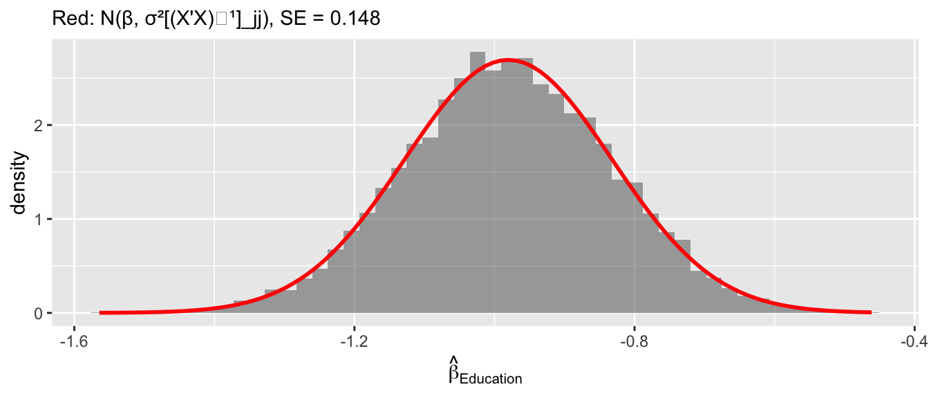

Diagnostic 2: $(n-K)s^2/\sigma^2 \sim \chi^2_{n-K}$.

df_chi <- n - K
c(simulated_mean = mean(sim$scaled_rss), theory_mean = df_chi,
  simulated_var  = var(sim$scaled_rss),  theory_var  = 2 * df_chi)

simulated_mean    theory_mean  simulated_var     theory_var 
          42.0           42.0           83.8           84.0

ggplot(sim, aes(scaled_rss)) +
  geom_histogram(aes(y = after_stat(density)), bins = 50, alpha = 0.5) +
  stat_function(fun = dchisq, args = list(df = df_chi),
                color = "red", linewidth = 1) +
  labs(subtitle = paste0("Red: χ²(", df_chi, ")"),
       x = expression((n-K)*s^2/sigma^2))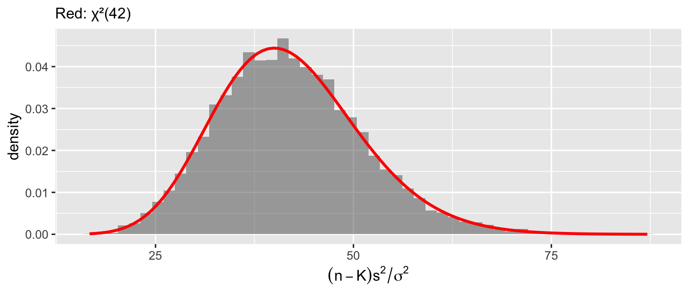

Diagnostic 3: $\hat\beta$ and $s^2$ are independent. Zero joint covariance plus joint normality implies independence — this is what lets us form the $t$-ratio.

cor(sim$bhat, sim$s2)

[1] 0.00725

Diagnostic 4: the studentized ratio follows $t_{n-K}$. Normal numerator over an independent scaled chi-squared denominator gives a $t$-distribution by definition.

\[T = \frac{\hat{\beta}_j - \beta_j}{\sqrt{s^2 [(X'X)^{-1}]_{jj}}} \sim t_{n-K} \tag{2}\]

ggplot(sim, aes(t)) +
  geom_histogram(aes(y = after_stat(density)), bins = 60, alpha = 0.5) +
  stat_function(fun = dt, args = list(df = n - K),
                color = "red", linewidth = 1) +
  stat_function(fun = dnorm, color = "blue", linewidth = 0.8, linetype = "dashed") +
  labs(subtitle = paste0("Red: t(", n-K, "). Blue dashed: N(0,1) — slightly thinner tails."),
       x = "t-statistic")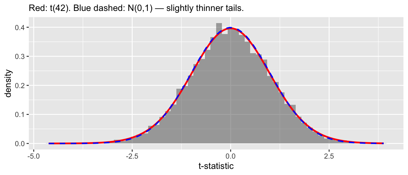

With $n - K = 42$ the $t$-distribution is close to normal but heavier-tailed — the extra uncertainty from estimating $\sigma^2$.

5 Applied inference with the Swiss data

5.1 The regression table

summary(mod)


Call:
lm(formula = Fertility ~ Education + Agriculture + Catholic + 
    Infant.Mortality, data = swiss)

Residuals:
    Min      1Q  Median      3Q     Max 
-14.676  -6.052   0.751   3.166  16.142 

Coefficients:
                 Estimate Std. Error t value Pr(>|t|)    
(Intercept)       62.1013     9.6049    6.47  8.5e-08 ***
Education         -0.9803     0.1481   -6.62  5.1e-08 ***
Agriculture       -0.1546     0.0682   -2.27   0.0286 *  
Catholic           0.1247     0.0289    4.31  9.5e-05 ***
Infant.Mortality   1.0784     0.3819    2.82   0.0072 ** 
---
Signif. codes:  0 '***' 0.001 '**' 0.01 '*' 0.05 '.' 0.1 ' ' 1

Residual standard error: 7.17 on 42 degrees of freedom
Multiple R-squared:  0.699, Adjusted R-squared:  0.671 
F-statistic: 24.4 on 4 and 42 DF,  p-value: 1.72e-10

Each row reports $\hat{\beta}_j$, $\text{SE}(\hat{\beta}_j)$, the $t$-statistic $\hat{\beta}_j / \text{SE}(\hat{\beta}_j)$ (testing $H_0: \beta_j = 0$), and the two-sided $p$-value.

5.2 Reading the output

The Education coefficient is $-0.98$ with SE $= 0.15$:

beta_hat <- coef(mod)["Education"]
se_hat <- sqrt(vcov(mod)["Education", "Education"])
t_stat <- beta_hat / se_hat
p_val <- 2 * (1 - pt(abs(t_stat), df = n - K))

c(estimate = beta_hat, se = se_hat, t = t_stat, p = p_val)

estimate.Education                 se        t.Education        p.Education 
         -9.80e-01           1.48e-01          -6.62e+00           5.14e-08

For each additional percentage point of post-primary education, fertility is about 1 point lower, and this is highly significant.

5.3 Confidence intervals

A $95\%$ confidence interval is $\hat{\beta}_j \pm t_{n-K, 0.975} \cdot \text{SE}(\hat{\beta}_j)$:

# Critical value from t-distribution
c_val <- qt(0.975, df = n - K)
c(critical_value = c_val, normal_approx = qnorm(0.975))

critical_value  normal_approx 
          2.02           1.96

# confint() does this automatically
confint(mod)

                   2.5 % 97.5 %
(Intercept)      42.7179 81.485
Education        -1.2792 -0.681
Agriculture      -0.2922 -0.017
Catholic          0.0664  0.183
Infant.Mortality  0.3078  1.849

# By hand for Education
ci_lo <- beta_hat - c_val * se_hat
ci_hi <- beta_hat + c_val * se_hat
c(lower = ci_lo, upper = ci_hi)

lower.Education upper.Education 
         -1.279          -0.681

The correct interpretation: $\beta$ is fixed, $\hat{C}$ is random. If we repeated this study many times, 95% of the computed intervals would cover the true $\beta$.

set.seed(7)
B_ci <- 50
beta_true_edu <- coef(mod)["Education"]

# Simulate: refit on Y drawn from the estimated model, compute CI each time
j_edu <- which(colnames(X) == "Education")
cv    <- qt(0.975, n - K)
ci_rows <- t(replicate(B_ci, {
  y_sim <- X %*% coef(mod) + rnorm(n, 0, sigma(mod))
  fit   <- lm.fit(X, y_sim)
  rss   <- sum(fit$residuals^2)
  xtxi  <- solve(crossprod(X))
  se    <- sqrt(rss / (n - K) * xtxi[j_edu, j_edu])
  est   <- unname(fit$coefficients[j_edu])
  c(est = est, lo = est - cv * se, hi = est + cv * se)
}))
ci_df <- data.frame(trial = 1:B_ci,
                    est = ci_rows[, "est"],
                    lo  = ci_rows[, "lo"],
                    hi  = ci_rows[, "hi"])
ci_df$miss <- ci_df$lo > beta_true_edu | ci_df$hi < beta_true_edu

ggplot(ci_df, aes(y = trial)) +
  geom_segment(aes(x = lo, xend = hi, yend = trial, color = miss),
               linewidth = 0.6) +
  geom_point(aes(x = est, color = miss), size = 1.2) +
  geom_vline(xintercept = beta_true_edu, color = "blue", linewidth = 0.8) +
  scale_color_manual(values = c("grey50", "#662a9b"),
                     labels = c("covers β", "misses β"), name = NULL) +
  labs(title = "50 simulated 95% CIs for β_Education",
       subtitle = "Blue line = true β. The interval is random; β is fixed.",
       x = expression(hat(beta)[Education]), y = "Simulation")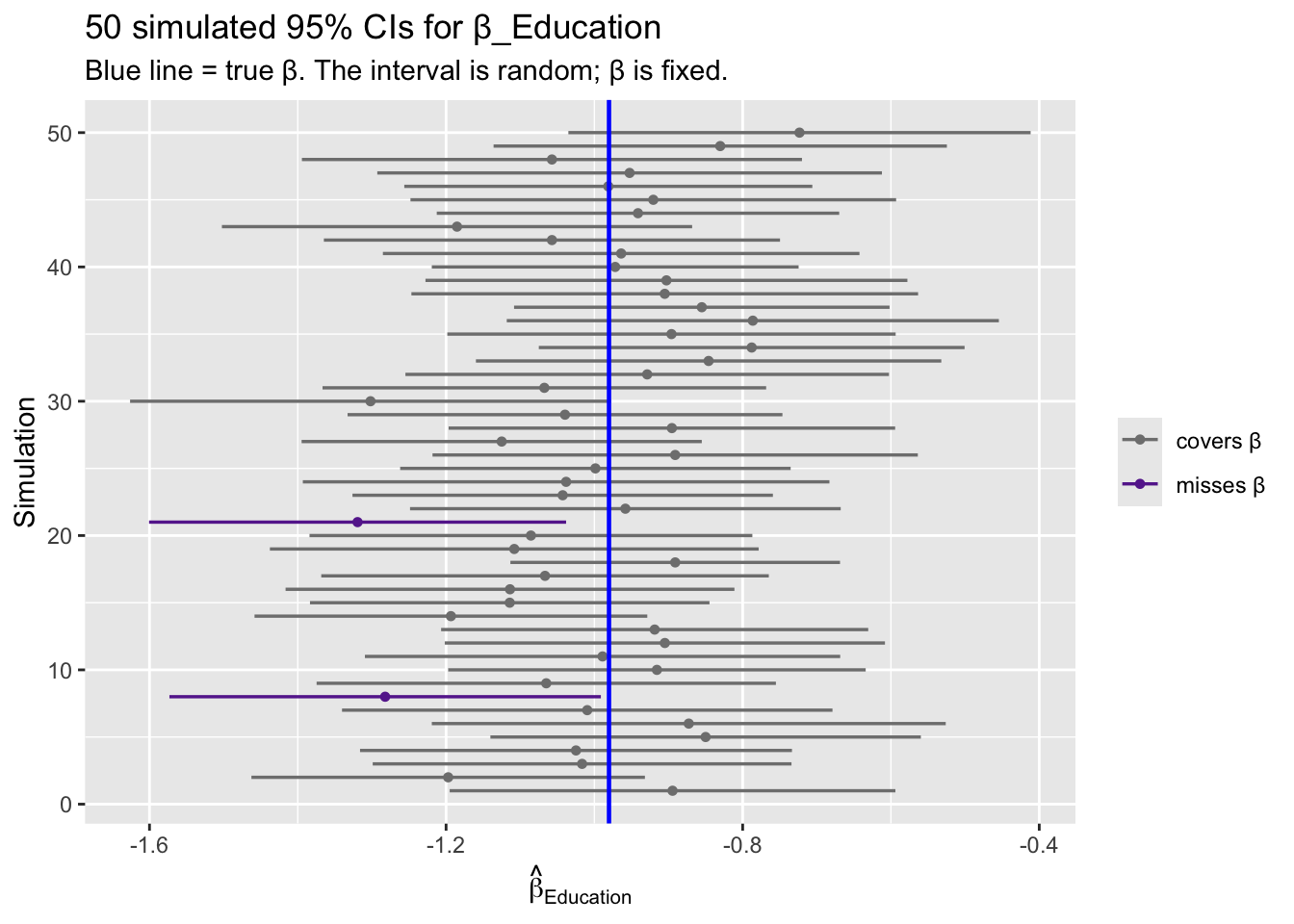

Each line is one CI from a resampled DGP. About 5% miss the truth (colored).

5.4 Robust confidence intervals

Under heteroskedasticity, the $t$-distribution is only approximate. Use lm_robust() or coeftest() with sandwich SEs:

# Robust SEs
mod_r <- lm_robust(Fertility ~ Education + Agriculture + Catholic + Infant.Mortality,
                    data = swiss, se_type = "HC2")

# Compare classical vs. robust CIs
ci_classical <- confint(mod)
ci_robust <- confint(mod_r)

data.frame(
  Variable = rownames(ci_classical),
  Classical_lo = ci_classical[, 1],
  Classical_hi = ci_classical[, 2],
  Robust_lo = ci_robust[, 1],
  Robust_hi = ci_robust[, 2]
)

                         Variable Classical_lo Classical_hi Robust_lo Robust_hi
(Intercept)           (Intercept)      42.7179       81.485   44.6132   79.5894
Education               Education      -1.2792       -0.681   -1.2837   -0.6769
Agriculture           Agriculture      -0.2922       -0.017   -0.2888   -0.0204
Catholic                 Catholic       0.0664        0.183    0.0681    0.1813
Infant.Mortality Infant.Mortality       0.3078        1.849    0.2865    1.8704

5.5 Visualizing confidence intervals

ci_df <- data.frame(
  term = rep(names(coef(mod))[-1], 2),
  estimate = rep(coef(mod)[-1], 2),
  lo = c(ci_classical[-1, 1], ci_robust[-1, 1]),
  hi = c(ci_classical[-1, 2], ci_robust[-1, 2]),
  type = rep(c("Classical", "HC2 Robust"), each = K - 1)
)

ggplot(ci_df, aes(x = estimate, y = term, color = type)) +
  geom_point(position = position_dodge(0.3)) +
  geom_errorbarh(aes(xmin = lo, xmax = hi),
                 height = 0.2, position = position_dodge(0.3)) +
  geom_vline(xintercept = 0, linetype = "dashed") +
  labs(title = "Swiss fertility: classical vs. robust confidence intervals",
       x = "Coefficient estimate", y = NULL, color = NULL)

Warning: `geom_errorbarh()` was deprecated in ggplot2 4.0.0.
ℹ Please use the `orientation` argument of `geom_errorbar()` instead.

`height` was translated to `width`.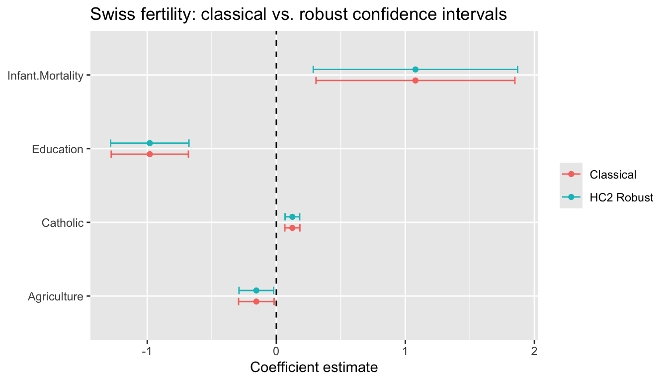

6 The $F$-test: when one $t$-test isn’t enough

The $t$-test handles one coefficient at a time. But many research questions involve several coefficients simultaneously, and the answer from testing them one-by-one can be misleading.

6.1 A motivating example: does training affect wages?

Suppose a job-training program’s effect depends on prior experience:

\[\text{Wage}_i = \beta_0 + \beta_1 \text{Train}_i + \beta_2 (\text{Train}_i \times \text{Exp}_i) + \beta_3 \text{Exp}_i + e_i\]

The effect of training at experience level Exp is $\beta_1 + \beta_2 \cdot \text{Exp}$ — it depends on both $\beta_1$ and $\beta_2$. To test whether training has any effect, we need $H_0: \beta_1 = 0 \text{ and } \beta_2 = 0$. A $t$-test on either coefficient alone tells us nothing about the joint claim.

set.seed(42)
n <- 80
experience <- runif(n, 1, 20)
training <- rbinom(n, 1, 0.5)
wage <- 10 + 3 * training + 0.5 * training * experience +
        0.8 * experience + rnorm(n, sd = 3)

full       <- lm(wage ~ training * experience)
restricted <- lm(wage ~ experience)

summary(full)$coefficients[c("training", "training:experience"), ]

                    Estimate Std. Error t value Pr(>|t|)
training               3.664      1.386    2.64 0.009958
training:experience    0.452      0.109    4.16 0.000083

Look at the $t$-statistic on training alone: the $p$-value is around $0.2$, nowhere near significant. If you only looked at that row, you might conclude training doesn’t matter.

6.2 The $F$-statistic as a comparison of fit

The $F$-test compares the restricted model (imposing $H_0$) to the unrestricted model:

\[F = \frac{(\tilde{e}'\tilde{e} - \hat{e}'\hat{e}) / q}{\hat{e}'\hat{e} / (n - K)} \sim F_{q,\, n-K} \quad\text{under } H_0 \tag{3}\]

Intuition: if $H_0$ is true, dropping the restricted variables shouldn’t hurt fit much. A large $F$ means the restricted model fits substantially worse — reject.

RSS_full   <- sum(resid(full)^2)
RSS_restr  <- sum(resid(restricted)^2)
q          <- 2
df_denom   <- df.residual(full)

F_stat <- ((RSS_restr - RSS_full) / q) / (RSS_full / df_denom)
p_F    <- pf(F_stat, q, df_denom, lower.tail = FALSE)
c(F = F_stat, df1 = q, df2 = df_denom, p = p_F)

       F      df1      df2        p 
1.03e+02 2.00e+00 7.60e+01 2.03e-22

anova(restricted, full)

Analysis of Variance Table

Model 1: wage ~ experience
Model 2: wage ~ training * experience
  Res.Df  RSS Df Sum of Sq   F Pr(>F)    
1     78 2201                            
2     76  591  2      1609 103 <2e-16 ***
---
Signif. codes:  0 '***' 0.001 '**' 0.01 '*' 0.05 '.' 0.1 ' ' 1

The joint test: $F \approx 39$, $p < 0.001$. Training clearly matters — the interaction absorbs much of the treatment effect, so neither coefficient looks impressive on its own. When a variable enters with an interaction, always test jointly.

6.3 Writing restrictions as $R\beta = r$

Any set of $q$ linear restrictions on $\beta$ can be written as $R\beta = r$. For $H_0: \beta_1 = 0 \text{ and } \beta_2 = 0$ in the training model:

\[\underbrace{\begin{pmatrix} 0 & 1 & 0 & 0 \\ 0 & 0 & 0 & 1 \end{pmatrix}}_{R}\, \underbrace{\begin{pmatrix}\beta_0\\ \beta_1\\ \beta_3\\ \beta_2\end{pmatrix}}_{\text{(intercept, training, experience, training:experience)}} = \begin{pmatrix}0\\0\end{pmatrix}\]

R orders main effects before interactions, so training:experience is the fourth coefficient. The $F$-statistic has an equivalent Wald form using only the unrestricted fit:

\[F = \frac{(R\hat\beta - r)'\,[R\,\hat{V}\,R']^{-1}\,(R\hat\beta - r)}{q}, \qquad \hat{V} = s^2 (X'X)^{-1}\]

R <- rbind(c(0, 1, 0, 0),
           c(0, 0, 0, 1))
r <- c(0, 0)

bhat <- coef(full)
Vhat <- vcov(full)
Rb_r <- R %*% bhat - r

F_wald <- as.numeric(t(Rb_r) %*% solve(R %*% Vhat %*% t(R)) %*% Rb_r / q)
c(F_wald = F_wald, F_RSS = F_stat)

F_wald  F_RSS 
   103    103

Identical. The Wald form is what you need when you move to robust or clustered covariance matrices — just swap $\hat{V}$.

6.4 `linearHypothesis()` does all of this

linearHypothesis(full, c("training = 0", "training:experience = 0"))


Linear hypothesis test:
training = 0
training:experience = 0

Model 1: restricted model
Model 2: wage ~ training * experience

  Res.Df  RSS Df Sum of Sq   F Pr(>F)    
1     78 2201                            
2     76  591  2      1609 103 <2e-16 ***
---
Signif. codes:  0 '***' 0.001 '**' 0.01 '*' 0.05 '.' 0.1 ' ' 1

6.5 $t^2 = F$ when $q = 1$

When a single restriction is tested, the $F$-statistic equals the square of the $t$-statistic:

t_exp <- summary(full)$coefficients["experience", "t value"]
F_exp <- linearHypothesis(full, "experience = 0")$F[2]
c(t_squared = t_exp^2, F = F_exp)

t_squared         F 
     91.9      91.9

6.6 Robust $F$-tests

Under heteroskedasticity, pass a robust covariance matrix:

linearHypothesis(full, c("training = 0", "training:experience = 0"),
                 vcov = vcovHC(full, type = "HC2"), test = "F")


Linear hypothesis test:
training = 0
training:experience = 0

Model 1: restricted model
Model 2: wage ~ training * experience

Note: Coefficient covariance matrix supplied.

  Res.Df Df   F Pr(>F)    
1     78                  
2     76  2 109 <2e-16 ***
---
Signif. codes:  0 '***' 0.001 '**' 0.01 '*' 0.05 '.' 0.1 ' ' 1

7 Prediction intervals

A confidence interval for $E[y \mid x_0]$ captures uncertainty about the regression line. A prediction interval for a new observation $y_0$ also includes the error variance $\sigma^2$:

\[\hat{y}_0 \pm t_{n-K, 1-\alpha/2} \cdot \sqrt{s^2 (1 + x_0'(X'X)^{-1}x_0)}\]

# Predict fertility for a district with median characteristics
new_data <- data.frame(
  Education  = median(swiss$Education),
  Agriculture = median(swiss$Agriculture),
  Catholic   = median(swiss$Catholic),
  Infant.Mortality = median(swiss$Infant.Mortality)
)

# Confidence interval for E[y|x]
predict(mod, newdata = new_data, interval = "confidence")

   fit  lwr  upr
1 69.4 66.6 72.1

# Prediction interval for a new y
predict(mod, newdata = new_data, interval = "prediction")

   fit  lwr  upr
1 69.4 54.6 84.1

The prediction interval is much wider — it accounts for the irreducible noise $\sigma^2$.

# Simple model for visualization
mod_simple <- lm(Fertility ~ Education, data = swiss)
pred_grid <- data.frame(Education = seq(1, 55, length.out = 100))
pred_ci <- predict(mod_simple, newdata = pred_grid, interval = "confidence")
pred_pi <- predict(mod_simple, newdata = pred_grid, interval = "prediction")

df_pred <- data.frame(
  Education = pred_grid$Education,
  fit = pred_ci[, 1],
  ci_lo = pred_ci[, 2], ci_hi = pred_ci[, 3],
  pi_lo = pred_pi[, 2], pi_hi = pred_pi[, 3]
)

ggplot() +
  geom_ribbon(data = df_pred, aes(Education, ymin = pi_lo, ymax = pi_hi),
              alpha = 0.15, fill = "steelblue") +
  geom_ribbon(data = df_pred, aes(Education, ymin = ci_lo, ymax = ci_hi),
              alpha = 0.3, fill = "steelblue") +
  geom_line(data = df_pred, aes(Education, fit), color = "steelblue", linewidth = 1) +
  geom_point(data = swiss, aes(Education, Fertility), alpha = 0.6) +
  labs(title = "Swiss fertility: confidence and prediction intervals",
       subtitle = "Dark band = CI for E[y|x], light band = PI for new observation",
       y = "Fertility")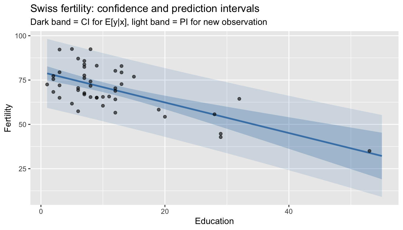

8 When do exact tests break down?

The $t$- and $F$-distributions are exact only under:

Normality of errors
Homoskedasticity
Known, correct model specification

What happens when errors are heteroskedastic? Compare the classical (homoskedastic) CI with the HC2 robust CI across sample sizes. DGP: slope $\beta_1 = 2$ with $e_i \sim N(0, 1 + x_i^2)$, so error variance grows with $x$.

set.seed(42)
B <- 2000
sample_sizes <- c(20, 50, 200)
beta_true <- 2

coverage_one <- function(nn) {
  cover_c <- cover_r <- logical(B)
  for (b in 1:B) {
    x <- rnorm(nn)
    e <- rnorm(nn, 0, sqrt(1 + x^2))
    y <- 1 + beta_true * x + e
    fit <- lm(y ~ x)
    cv  <- qt(0.975, nn - 2)

    se_c <- sqrt(vcov(fit)["x", "x"])
    se_r <- sqrt(vcovHC(fit, type = "HC2")["x", "x"])
    b_x  <- coef(fit)["x"]

    cover_c[b] <- abs(b_x - beta_true) < cv * se_c
    cover_r[b] <- abs(b_x - beta_true) < cv * se_r
  }
  c(Classical = mean(cover_c), HC2 = mean(cover_r))
}

results <- cbind(n = sample_sizes,
                 as.data.frame(t(sapply(sample_sizes, coverage_one))))
results

    n Classical   HC2
1  20     0.848 0.896
2  50     0.857 0.932
3 200     0.849 0.948

HC2 maintains near-nominal coverage across all sample sizes. Classical CIs undercover — they ignore that variance grows with $x$, so $s^2 (X'X)^{-1}$ misstates the sampling variance of $\hat\beta$. The bootstrap offers a third alternative, discussed in Chapter 8.

9 Summary

Concept	Formula	R code
Log-likelihood	$\ell = -\frac{n}{2}\log(2\pi\sigma^2) - \frac{1}{2\sigma^2}\sum e_i^2$	`logLik(mod)`
MLE of $\beta$	$(X'X)^{-1}X'y$ (= OLS)	`coef(lm(...))`
MLE of $\sigma^2$	$\frac{1}{n}\sum \hat{e}_i^2$ (biased)	`sum(resid(mod)^2) / n`
AIC / BIC	$-2\ell + 2K$ / $-2\ell + K\log n$	`AIC(mod)`, `BIC(mod)`
$t$-statistic	$\hat{\beta}_j / \text{SE}(\hat{\beta}_j) \sim t_{n-K}$	`summary(mod)$coefficients`
Confidence interval	$\hat{\beta}_j \pm t_{n-K,\,0.975} \cdot \text{SE}$	`confint(mod)`
$F$-test	$\frac{(RSS_R - RSS_U)/q}{RSS_U/(n-K)} \sim F_{q,n-K}$	`anova(mod_r, mod_u)`
Joint hypothesis	$R\beta = r$	`linearHypothesis(mod, ...)`
Robust $F$-test	—	`linearHypothesis(mod, ..., vcov = vcovHC)`
Prediction interval	$\hat{y}_0 \pm t \cdot s\sqrt{1 + x_0'(X'X)^{-1}x_0}$	`predict(mod, interval = "prediction")`

Key takeaway. The normal linear model gives us exact finite-sample distributions: $\hat{\beta}$ is normal, $s^2$ is chi-squared, their ratio gives $t$, and nested model comparisons give $F$. These are the foundation of every regression table. But they rely on normality and homoskedasticity — when those fail, use robust SEs and asymptotic theory instead.

6. Small Sample Inference

1 Likelihood

1.1 Example: binomial likelihood

1.2 The log-likelihood

1.3 Score, Hessian, and Fisher information

2 The normal linear model

2.1 Writing the log-likelihood in R

2.2 MLE = OLS

2.3 `logLik()` and model comparison

3 Scores as moment conditions

4 Exact distributions under normality

4.1 One simulation, four diagnostics

5 Applied inference with the Swiss data

5.1 The regression table

5.2 Reading the output

5.3 Confidence intervals

5.4 Robust confidence intervals

5.5 Visualizing confidence intervals

6 The \(F\)-test: when one \(t\)-test isn’t enough

6.1 A motivating example: does training affect wages?

6.2 The \(F\)-statistic as a comparison of fit

6.3 Writing restrictions as \(R\beta = r\)

6.4 `linearHypothesis()` does all of this

6.5 \(t^2 = F\) when \(q = 1\)

6.6 Robust \(F\)-tests

7 Prediction intervals

8 When do exact tests break down?

9 Summary

1 Likelihood

1.1 Example: binomial likelihood

1.2 The log-likelihood

1.3 Score, Hessian, and Fisher information

2 The normal linear model

2.1 Writing the log-likelihood in R

2.2 MLE = OLS

2.3 logLik() and model comparison

3 Scores as moment conditions

4 Exact distributions under normality

4.1 One simulation, four diagnostics

5 Applied inference with the Swiss data

5.1 The regression table

5.2 Reading the output

5.3 Confidence intervals

5.4 Robust confidence intervals

5.5 Visualizing confidence intervals

6 The \(F\)-test: when one \(t\)-test isn’t enough

6.1 A motivating example: does training affect wages?

6.2 The \(F\)-statistic as a comparison of fit

6.3 Writing restrictions as \(R\beta = r\)

6.4 linearHypothesis() does all of this

6.5 \(t^2 = F\) when \(q = 1\)

6.6 Robust \(F\)-tests

7 Prediction intervals

8 When do exact tests break down?

9 Summary

2.3 `logLik()` and model comparison

6.4 `linearHypothesis()` does all of this