library(ggplot2)
library(MASS)
library(sandwich)
library(lmtest)
library(estimatr)
library(carData)
data(Prestige)
options(digits = 3)
tr <- function(M) sum(diag(M))5. Efficiency and GLS
Weighted least squares, feasible GLS, and the method of moments
When error variances differ across observations, OLS is still unbiased but no longer efficient. This chapter develops WLS and GLS as the natural response: weight observations by their precision. We build everything from matrix algebra, connect the estimator to the method of moments, and implement feasible GLS when the variance structure must be estimated from data. Along the way we introduce the sandwich and estimatr packages — the practical tools for robust inference in R.
Questions this chapter answers:
- Why are classical standard errors wrong under heteroskedasticity, and what does the sandwich formula fix?
- How do WLS and GLS improve efficiency by weighting observations by their precision?
- When should you use FGLS vs. simply reporting robust standard errors?
- What is the connection between HC0/HC1/HC2/HC3 and the leverage-corrected residual types?
1 The variance of OLS under non-spherical errors
Recall the OLS estimator: \(\hat{\beta} = \beta + (X'X)^{-1}X'e\). The variance is:
\[\text{Var}[\hat{\beta} \mid X] = (X'X)^{-1} X' \text{Var}[e \mid X] \, X (X'X)^{-1}\]
Under homoskedasticity (\(\text{Var}[e \mid X] = \sigma^2 I\)), this simplifies to \(\sigma^2(X'X)^{-1}\). But when \(\text{Var}[e \mid X] = \Omega \neq \sigma^2 I\), we get the sandwich formula:
\[(X'X)^{-1} (X' \Omega X) (X'X)^{-1} \tag{1}\]
The “bread” is \((X'X)^{-1}\) and the “meat” is \(X'\Omega X = \sum_{i=1}^n \sigma_i^2 x_i x_i'\). Let’s see what happens when we ignore heteroskedasticity and use the classical formula anyway.
Definition 1 (Sandwich Variance Estimator) Under heteroskedasticity (\(\text{Var}[e|X] = \Omega \neq \sigma^2 I\)), the variance of OLS is \((X'X)^{-1}(X'\Omega X)(X'X)^{-1}\). The HC estimators replace \(\Omega\) with diagonal matrices of squared residuals, possibly adjusted for leverage.
1.1 Example: when classical standard errors lie
We design a DGP with strong heteroskedasticity: the error standard deviation grows as \(x^2\), so variance ranges from 1 (at \(x = 1\)) to 10,000 (at \(x = 10\)). This makes the problem impossible to miss.
set.seed(42)
n <- 200
x <- runif(n, 1, 10)
X <- cbind(1, x)

# Strongly heteroskedastic DGP: SD = x^2
sigma_i <- x^2   # variance = x^4, ratio of 10000:1
y <- 2 + 3 * x + rnorm(n, 0, sigma_i)
mod <- lm(y ~ x)
First, let’s build the sandwich by hand to see the matrix algebra:
# Classical variance: s^2 * (X'X)^{-1}
s2 <- sum(resid(mod)^2) / (n - 2)
V_classical <- s2 * solve(crossprod(X))

# Sandwich variance (HC0): (X'X)^{-1} X' diag(e^2) X (X'X)^{-1}
e_hat <- resid(mod)
bread <- solve(crossprod(X))
meat <- t(X) %*% diag(e_hat^2) %*% X
V_HC0 <- bread %*% meat %*% bread

# Compare standard errors for the slope
c(classical = sqrt(V_classical[2, 2]),
  HC0       = sqrt(V_HC0[2, 2]))
classical HC0
1.31 1.48 Now the practical way — sandwich::vcovHC() computes this in one line:
# HC0 (White's original)
sqrt(diag(vcovHC(mod, type = "HC0")))
(Intercept) x
5.48 1.48 # HC1 (small-sample correction: multiply by n/(n-k))
sqrt(diag(vcovHC(mod, type = "HC1")))(Intercept) x
5.51 1.49 # HC2 (adjusts for leverage)
sqrt(diag(vcovHC(mod, type = "HC2")))(Intercept) x
5.52 1.49 # HC3 (jackknife — recommended default for linear regression)
sqrt(diag(vcovHC(mod, type = "HC3")))(Intercept) x
5.56 1.50 The four variants differ in how they scale the squared residuals in the sandwich meat:
| Variant | Meat diagonal | Intuition |
|---|---|---|
| HC0 | \(\hat{e}_i^2\) | White’s original — no correction |
| HC1 | \(\frac{n}{n-K}\hat{e}_i^2\) | Degrees-of-freedom correction (Stata’s default) |
| HC2 | \(\frac{\hat{e}_i^2}{1-h_{ii}}\) | Unbiases \(\hat{e}_i^2\) for leverage |
| HC3 | \(\frac{\hat{e}_i^2}{(1-h_{ii})^2}\) | Jackknife — more conservative at high leverage |
HC3 is equivalent to the jackknife (leave-one-out) variance estimator for OLS. Compared to HC2 (which exactly unbiases \(\hat{e}_i^2\)), HC3 applies an extra \((1-h_{ii})^{-1}\) factor that further inflates SEs at high-leverage points. This conservatism improves finite-sample coverage — Long and Ervin (2000) showed HC3 has the best coverage among the HC variants, especially when \(n\) is moderate and leverage is uneven.
Or even simpler — estimatr::lm_robust() fits the model and computes robust SEs in one step. Note that estimatr defaults to HC2; pass se_type = "HC3" for the jackknife:
mod_robust <- lm_robust(y ~ x, se_type = "HC3")
summary(mod_robust)
Call:
lm_robust(formula = y ~ x, se_type = "HC3")

Standard error type:  HC3

Coefficients:
            Estimate Std. Error t value Pr(>|t|) CI Lower CI Upper  DF
(Intercept)     4.07       5.56   0.732    0.465   -6.891    15.02 198
x               2.30       1.50   1.530    0.128   -0.664     5.26 198

Multiple R-squared:  0.0154 ,   Adjusted R-squared:  0.0104
F-statistic: 2.34 on 1 and 198 DF,  p-value: 0.128
Compare the standard errors side by side:
se_table <- data.frame(
  Classical = summary(mod)$coefficients[, 2],
  HC0 = sqrt(diag(vcovHC(mod, type = "HC0"))),
  HC1 = sqrt(diag(vcovHC(mod, type = "HC1"))),
  HC2 = sqrt(diag(vcovHC(mod, type = "HC2"))),
  HC3 = sqrt(diag(vcovHC(mod, type = "HC3"))),
  row.names = c("(Intercept)", "x")
)
round(se_table, 3)
Classical HC0 HC1 HC2 HC3
(Intercept) 8.20 5.48 5.51 5.52 5.56
x 1.31 1.48 1.49 1.49 1.50The classical SE for the slope is far too small — it ignores that the high-\(x\) observations (which pull the slope) are exactly the noisiest ones. HC3 is the most conservative and closest to the true sampling variability.
WarningClassical Standard Errors Can Be Dangerously Wrong
Under heteroskedasticity, classical SEs can be too small by a factor of 2 or more, producing confidence intervals with far below nominal coverage. Always use robust SEs (HC3) as the default for cross-sectional linear regression.
df <- data.frame(x = x, residual = resid(mod))
ggplot(df, aes(x, residual)) +
  geom_point(alpha = 0.4) +
  geom_hline(yintercept = 0, linetype = "dashed") +
  labs(title = "Residuals fan out dramatically with x",
       subtitle = "SD grows as x², so variance ratio is 10000:1")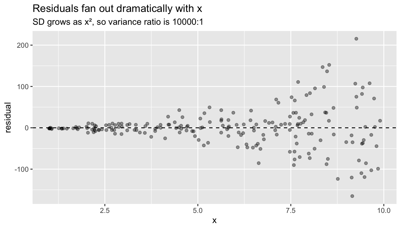
1.2 Monte Carlo: coverage of classical vs. robust intervals
set.seed(1)
B <- 2000
cover_classical <- cover_HC0 <- cover_HC2 <- cover_HC3 <- logical(B)
beta_true <- 3

for (b in 1:B) {
  x_sim <- runif(n, 1, 10)
  X_sim <- cbind(1, x_sim)
  sigma_sim <- x_sim^2
  y_sim <- 2 + beta_true * x_sim + rnorm(n, 0, sigma_sim)

  fit <- lm(y_sim ~ x_sim)
  b_hat <- coef(fit)[2]

  # Classical CI
  se_class <- summary(fit)$coefficients[2, 2]
  ci_class <- b_hat + c(-1, 1) * 1.96 * se_class
  cover_classical[b] <- ci_class[1] < beta_true & beta_true < ci_class[2]

  # HC0 (White)
  se_hc0 <- sqrt(vcovHC(fit, type = "HC0")[2, 2])
  ci_hc0 <- b_hat + c(-1, 1) * 1.96 * se_hc0
  cover_HC0[b] <- ci_hc0[1] < beta_true & beta_true < ci_hc0[2]

  # HC2
  se_hc2 <- sqrt(vcovHC(fit, type = "HC2")[2, 2])
  ci_hc2 <- b_hat + c(-1, 1) * 1.96 * se_hc2
  cover_HC2[b] <- ci_hc2[1] < beta_true & beta_true < ci_hc2[2]

  # HC3 (jackknife)
  se_hc3 <- sqrt(vcovHC(fit, type = "HC3")[2, 2])
  ci_hc3 <- b_hat + c(-1, 1) * 1.96 * se_hc3
  cover_HC3[b] <- ci_hc3[1] < beta_true & beta_true < ci_hc3[2]
}

c(classical = mean(cover_classical),
  HC0       = mean(cover_HC0),
  HC2       = mean(cover_HC2),
  HC3       = mean(cover_HC3))
classical HC0 HC2 HC3
0.894 0.953 0.954 0.955 Classical intervals have terrible coverage. HC0 and HC2 improve but still undercover. HC3 gets closest to the nominal 95% — the extra conservatism of the jackknife pays off when leverage is uneven, as it is here (high-\(x\) observations have both high variance and high leverage).
1.3 lm_robust vs. coeftest: two workflows
In practice, there are two ways to get robust inference. Use whichever fits your workflow:
# Workflow 1: estimatr — one function does everything
mod_r <- lm_robust(y ~ x, se_type = "HC3")
coef(summary(mod_r))
Estimate Std. Error t value Pr(>|t|) CI Lower CI Upper DF
(Intercept) 4.07 5.56 0.732 0.465 -6.891 15.02 198
x 2.30 1.50 1.530 0.128 -0.664 5.26 198# Workflow 2: sandwich + lmtest — post-hoc correction to a fitted lm
coeftest(mod, vcov = vcovHC(mod, type = "HC3"))
t test of coefficients:

            Estimate Std. Error t value Pr(>|t|)
(Intercept)     4.07       5.56    0.73     0.47
x               2.30       1.50    1.53     0.13
The coeftest() approach is useful when you’ve already fit a model with lm() and want to report robust SEs. lm_robust() is cleaner when you know from the start that you want robust inference.
2 Weighted least squares
The sandwich formula tells us what the variance is. But can we do better than OLS? Yes — if we know (or can estimate) the variance structure, we should exploit it.
2.1 The idea: weight by precision
If observation \(i\) has variance \(\sigma_i^2\), it carries less information than an observation with variance \(\sigma_j^2 < \sigma_i^2\). WLS weights each observation by \(w_i = 1/\sigma_i^2\), downweighting noisy observations:
\[\hat{\beta}_{WLS} = \arg\min_\beta \sum_{i=1}^n w_i (y_i - x_i'\beta)^2 = (X'WX)^{-1} X'Wy \tag{2}\]
where \(W = \text{diag}(w_1, \ldots, w_n)\).
2.2 Two-group example
Suppose we survey two groups: Group A (\(n_A = 100\), \(\sigma_A = 10\)) and Group B (\(n_B = 100\), \(\sigma_B = 1\)). OLS gives equal weight to every observation. WLS gives Group A weight \(1/100\) and Group B weight \(1\).
set.seed(99)
B <- 5000
b_ols <- b_wls <- numeric(B)

for (i in 1:B) {
  x_sim <- rnorm(200)
  sigma_sim <- c(rep(10, 100), rep(1, 100))
  y_sim <- 1 + 2 * x_sim + rnorm(200, 0, sigma_sim)

  b_ols[i] <- coef(lm(y_sim ~ x_sim))[2]
  b_wls[i] <- coef(lm(y_sim ~ x_sim, weights = 1 / sigma_sim^2))[2]
}

# Both unbiased, but WLS has much lower variance
c(bias_ols = mean(b_ols) - 2, bias_wls = mean(b_wls) - 2)
bias_ols bias_wls
-0.00434 -0.00125 c(sd_ols = sd(b_ols), sd_wls = sd(b_wls))sd_ols sd_wls
0.507 0.103 Both estimators are unbiased, but WLS standard errors are dramatically smaller. GLS is just common sense: trust precise observations more.
df_sim <- data.frame(
  estimate = c(b_ols, b_wls),
  method = rep(c("OLS", "WLS"), each = B)
)
ggplot(df_sim, aes(estimate, fill = method)) +
  geom_density(alpha = 0.4) +
  geom_vline(xintercept = 2, linetype = "dashed") +
  labs(title = "OLS vs. WLS sampling distributions",
       subtitle = "Both centered on truth, but WLS is much tighter",
       x = expression(hat(beta)))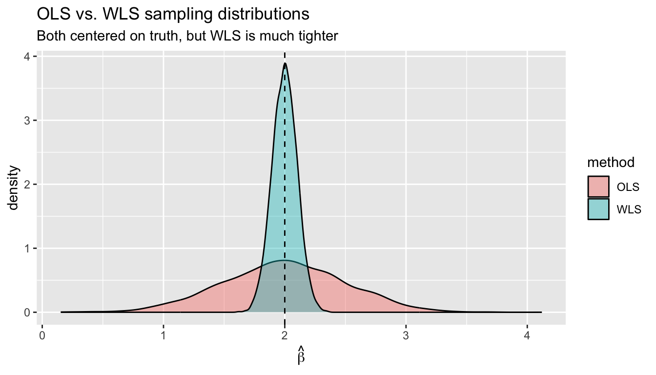
2.3 WLS in R: lm(..., weights = )
mod_ols <- lm(prestige ~ education + income + women, data = Prestige)

# Suppose we know variance is proportional to income
# (higher-income occupations have more variable prestige)
w <- 1 / Prestige$income
mod_wls <- lm(prestige ~ education + income + women, data = Prestige, weights = w)

# Compare coefficients
cbind(OLS = coef(mod_ols), WLS = coef(mod_wls))
OLS WLS
(Intercept) -6.79433 -9.97061
education 4.18664 3.18162
income 0.00131 0.00303
women -0.00891 0.07049The interpretation: each coefficient gives the predicted change in prestige for a one-unit increase in that variable, holding the others constant. Under OLS, a one-year increase in average education is associated with about 4.2 more prestige points. Under WLS (weighting by \(1/\text{income}\)), the education coefficient shifts to 3.2 — WLS gives more influence to low-income occupations (which get weight \(w_i = 1/\text{income}_i\)), and in this group education may matter more for prestige. The income coefficient is small in both cases because income is in dollars: a $1,000 increase predicts about 1.3 prestige points under OLS. The coefficient on women (percent female) is negative in both, reflecting a well-known pattern: more female-dominated occupations tend to have lower prestige scores, conditional on education and income.
The key point is that WLS changes the point estimates, not just the standard errors. It answers a subtly different question: “what is the relationship, weighting observations by their precision?”
2.4 WLS as a transformed regression
WLS is equivalent to pre-multiplying the model by \(W^{1/2}\):
\[W^{1/2} y = W^{1/2} X \beta + W^{1/2} e\]
The transformed errors have variance \(W^{1/2} \Omega W^{1/2} = I\) (if \(W = \Omega^{-1}\)), so OLS on the transformed data is efficient. Let’s verify:
# Manual transformation
W_half <- diag(sqrt(w))
y_tilde <- W_half %*% Prestige$prestige
X_raw <- cbind(1, Prestige$education, Prestige$income, Prestige$women)
X_tilde <- W_half %*% X_raw

# OLS on transformed data
beta_transformed <- solve(crossprod(X_tilde)) %*% crossprod(X_tilde, y_tilde)

# Compare to lm(..., weights = )
all.equal(as.numeric(beta_transformed), as.numeric(coef(mod_wls)))
[1] TRUEThe transformation approach makes clear what weights does: it rescales each observation so that the transformed errors are homoskedastic.
Important note on the intercept. After transformation, the column of ones becomes \(W^{1/2} \mathbf{1} = (\sqrt{w_1}, \ldots, \sqrt{w_n})'\), which is no longer constant. If you run the transformed regression manually, you must suppress the automatic intercept and include the transformed constant as a regressor:
# Transformed data
df_t <- data.frame(
  y = as.numeric(y_tilde),
  const = as.numeric(W_half %*% rep(1, nrow(Prestige))),
  education = as.numeric(W_half %*% Prestige$education),
  income = as.numeric(W_half %*% Prestige$income),
  women = as.numeric(W_half %*% Prestige$women)
)

# -1 suppresses R's intercept; 'const' is the transformed intercept
mod_manual <- lm(y ~ const + education + income + women - 1, data = df_t)
all.equal(as.numeric(coef(mod_manual)), as.numeric(coef(mod_wls)))
[1] TRUE3 GLS: The general transformation
WLS handles the case where \(\Omega\) is diagonal (heteroskedasticity only). GLS handles the general case where errors may also be correlated. The key idea is the same: find a transformation \(\Omega^{-1/2}\) that sphericizes the errors.
3.1 Eigendecomposition of \(\Omega\)
Any positive definite symmetric matrix can be factored as \(\Omega = C \Lambda C'\), where \(C\) is the matrix of eigenvectors and \(\Lambda\) is diagonal with eigenvalues. Then:
\[\Omega^{-1/2} = C \Lambda^{-1/2} C'\]
# A small example: 4x4 covariance matrix with correlation
n_small <- 4
rho <- 0.6
Omega_small <- rho^abs(outer(1:n_small, 1:n_small, "-"))  # AR(1) structure
Omega_small
[,1] [,2] [,3] [,4]
[1,] 1.000 0.60 0.36 0.216
[2,] 0.600 1.00 0.60 0.360
[3,] 0.360 0.60 1.00 0.600
[4,] 0.216 0.36 0.60 1.000eig <- eigen(Omega_small)
C <- eig$vectors
Lambda <- diag(eig$values)
# Omega^{-1/2}
Omega_inv_half <- C %*% diag(1 / sqrt(eig$values)) %*% t(C)
# Verify: Omega^{-1/2} Omega Omega^{-1/2} = I
all.equal(Omega_inv_half %*% Omega_small %*% Omega_inv_half, diag(n_small),
check.attributes = FALSE)[1] TRUE3.2 GLS formula
The GLS estimator pre-multiplies by \(\Omega^{-1/2}\), then applies OLS:
\[\hat{\beta}_{GLS} = (X'\Omega^{-1}X)^{-1} X'\Omega^{-1}y \tag{3}\]
Its variance is \(\sigma^2(X'\Omega^{-1}X)^{-1}\), which is the efficiency lower bound — no other linear unbiased estimator can do better.
Theorem 1 (GLS Estimator) The GLS estimator \(\hat\beta_{GLS} = (X'\Omega^{-1}X)^{-1}X'\Omega^{-1}y\) is the best linear unbiased estimator (BLUE) when \(\text{Var}[e|X] = \sigma^2\Omega\). Its variance \(\sigma^2(X'\Omega^{-1}X)^{-1}\) achieves the efficiency lower bound among linear unbiased estimators.
Theorem 2 (Gauss-Markov Theorem) Under the assumptions \(\mathbb{E}[e|X] = 0\) and \(\text{Var}[e|X] = \sigma^2 I\) (homoskedasticity), OLS is BLUE — the Best Linear Unbiased Estimator. No other linear unbiased estimator has smaller variance. When homoskedasticity fails, GLS replaces OLS as BLUE.
3.3 Monte Carlo: GLS with correlated errors
set.seed(7)
n <- 80
rho <- 0.8

# AR(1) correlation matrix
Omega <- rho^abs(outer(1:n, 1:n, "-"))
Omega_inv <- solve(Omega)

# Cholesky factor for generating correlated errors
L <- t(chol(Omega))

x <- sort(runif(n, 0, 10))
X <- cbind(1, x)
beta_true <- c(1, 2)

B <- 3000
b_ols <- b_gls <- matrix(NA, B, 2)

for (b in 1:B) {
  e <- L %*% rnorm(n)  # correlated errors
  y_sim <- X %*% beta_true + e

  b_ols[b, ] <- as.numeric(solve(crossprod(X)) %*% crossprod(X, y_sim))
  b_gls[b, ] <- as.numeric(solve(t(X) %*% Omega_inv %*% X) %*%
                              (t(X) %*% Omega_inv %*% y_sim))
}

# Both unbiased
colMeans(b_ols) - beta_true
[1] 0.01416 -0.00327colMeans(b_gls) - beta_true[1] 0.01215 -0.00282# But GLS is more efficient (lower SD for slope)
c(sd_ols_slope = sd(b_ols[, 2]), sd_gls_slope = sd(b_gls[, 2]))sd_ols_slope sd_gls_slope
0.109 0.101 df_ar <- data.frame(
slope = c(b_ols[, 2], b_gls[, 2]),
method = rep(c("OLS", "GLS"), each = B)
)
ggplot(df_ar, aes(slope, fill = method)) +
geom_density(alpha = 0.4) +
geom_vline(xintercept = 2, linetype = "dashed") +
labs(title = "OLS vs. GLS with AR(1) errors (ρ = 0.8)",
subtitle = "GLS recovers the efficiency lost to serial correlation",
x = expression(hat(beta)[1]))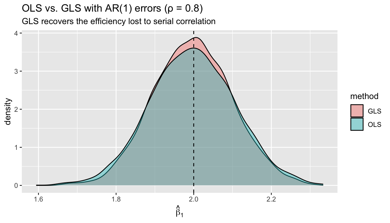
3.4 The GLS projection matrix
In Chapter 3, we studied \(P = X(X'X)^{-1}X'\). The GLS analog replaces the inner product:
\[P_{GLS} = X(X'\Omega^{-1}X)^{-1}X'\Omega^{-1}\]
Unlike the OLS projection, \(P_{GLS}\) is not symmetric — but it is still idempotent:
P_gls <- X %*% solve(t(X) %*% Omega_inv %*% X) %*% t(X) %*% Omega_inv

# Not symmetric
max(abs(P_gls - t(P_gls)))
[1] 0.272# But idempotent
all.equal(P_gls %*% P_gls, P_gls)[1] TRUE4 Feasible GLS
GLS requires knowing \(\Omega\). In practice, we never know the true variance structure. Feasible GLS (FGLS) estimates \(\Omega\) from the data in a first step, then applies GLS with \(\hat{\Omega}\).
4.1 Step-by-step FGLS for heteroskedasticity
The most common approach assumes a multiplicative heteroskedasticity model:
\[\sigma_i^2 = \text{Var}[e_i \mid x_i] = \exp(\gamma_0 + \gamma_1 z_i)\]
where \(z_i\) is some function of \(x_i\).
set.seed(42)
n <- 300

# DGP: variance depends strongly on x
x <- runif(n, 1, 10)
sigma_true <- exp(0.5 + 0.3 * x)  # log-linear variance
y <- 2 + 3 * x + rnorm(n) * sqrt(sigma_true)

# Step 1: Run OLS, save residuals
mod_step1 <- lm(y ~ x)

# Step 2: Regress log(e^2) on x to estimate the variance function
log_e2 <- log(resid(mod_step1)^2)
mod_var <- lm(log_e2 ~ x)

# Step 3: Predicted variances -> weights
sigma2_hat <- exp(fitted(mod_var))
w_fgls <- 1 / sigma2_hat

# Step 4: Run WLS with estimated weights
mod_fgls <- lm(y ~ x, weights = w_fgls)

cbind(OLS = coef(mod_step1), FGLS = coef(mod_fgls), Truth = c(2, 3))
OLS FGLS Truth
(Intercept) 1.85 2.03 2
x 3.02 2.98 3Compare standard errors — OLS classical, OLS with HC3, and FGLS:
X_fgls <- cbind(1, x)

se_compare <- data.frame(
  OLS_classical = summary(mod_step1)$coefficients[, 2],
  OLS_HC3       = sqrt(diag(vcovHC(mod_step1, type = "HC3"))),
  FGLS          = summary(mod_fgls)$coefficients[, 2],
  row.names = c("(Intercept)", "x")
)
round(se_compare, 4)
OLS_classical OLS_HC3 FGLS
(Intercept) 0.4559 0.3659 0.255
x 0.0753 0.0891 0.062HC3 corrects the SE without changing the point estimate. FGLS changes both — it re-estimates \(\hat{\beta}\) using the variance information, gaining efficiency.
4.2 Implementing FGLS with matrix algebra
X_mat <- cbind(1, x)
Omega_hat_inv <- diag(1 / sigma2_hat)

# GLS formula with estimated Omega
beta_fgls <- solve(t(X_mat) %*% Omega_hat_inv %*% X_mat) %*%
             (t(X_mat) %*% Omega_hat_inv %*% y)

all.equal(as.numeric(beta_fgls), as.numeric(coef(mod_fgls)))
[1] TRUE4.3 How well does FGLS estimate the variance function?
df_var <- data.frame(
  x = x,
  log_e2 = log_e2,
  fitted_log_var = fitted(mod_var),
  true_log_var = 0.5 + 0.3 * x
)

ggplot(df_var, aes(x)) +
  geom_point(aes(y = log_e2), alpha = 0.2, size = 1) +
  geom_line(aes(y = fitted_log_var, color = "Estimated"), linewidth = 1) +
  geom_line(aes(y = true_log_var, color = "True"), linewidth = 1, linetype = "dashed") +
  labs(title = "FGLS variance function estimation",
       subtitle = "Regressing log(ê²) on x recovers the variance structure",
       y = "log(σ²)", color = NULL)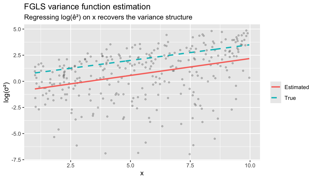
4.4 Monte Carlo: OLS vs. FGLS efficiency
set.seed(2)
B <- 2000
b_ols_mc <- b_fgls_mc <- numeric(B)

for (b in 1:B) {
  x_mc <- runif(n, 1, 10)
  sigma_mc <- exp(0.5 + 0.3 * x_mc)
  y_mc <- 2 + 3 * x_mc + rnorm(n) * sqrt(sigma_mc)

  # OLS
  fit_ols <- lm(y_mc ~ x_mc)
  b_ols_mc[b] <- coef(fit_ols)[2]

  # FGLS
  log_e2_mc <- log(resid(fit_ols)^2)
  sigma2_hat_mc <- exp(fitted(lm(log_e2_mc ~ x_mc)))
  b_fgls_mc[b] <- coef(lm(y_mc ~ x_mc, weights = 1 / sigma2_hat_mc))[2]
}

c(sd_ols = sd(b_ols_mc), sd_fgls = sd(b_fgls_mc),
  efficiency_gain = sd(b_ols_mc) / sd(b_fgls_mc))
sd_ols sd_fgls efficiency_gain
0.0841 0.0687 1.2255 Even though FGLS must estimate the weights, it still substantially improves on OLS when the heteroskedasticity is strong.
NoteFGLS Requires a Correct Variance Model
FGLS gains efficiency over OLS + robust SEs only when the variance model is correctly specified. If \(\hat\Omega\) is misspecified, FGLS point estimates are still consistent but may be less efficient than OLS, and its reported SEs may be wrong. Use FGLS only when you have a substantive reason to model the variance.
5 Two strategies for heteroskedasticity
You have two options when errors may be heteroskedastic:
- Robust SEs (agnostic). Keep the OLS point estimates and correct only the standard errors with the sandwich formula. Requires no model for the variance — always valid.
- WLS/FGLS (model-based). Specify a model for the variance, estimate it, and re-weight. More efficient if the variance model is correct; potentially worse if it’s misspecified.
A common older workflow was to first test for heteroskedasticity (Breusch-Pagan, White’s test), then decide whether to apply WLS. This is pre-testing — using the same data to choose the estimator and then to estimate — and it distorts the sampling distribution of the final estimate. The resulting “test, then decide” procedure is neither the OLS distribution nor the WLS distribution; its true coverage and size are hard to characterize.
The modern recommendation: always report robust SEs (HC3 by default for linear regression). Use WLS/FGLS only when you have a substantive reason to model the variance — for instance, when observations are group averages with known group sizes, or when a theoretical model predicts the variance form. The decision to use WLS should come from domain knowledge, not from a hypothesis test on the same data.
5.1 The Breusch-Pagan test (for understanding, not for pre-testing)
The Breusch-Pagan test is still useful as a descriptive diagnostic — it tells you whether your residuals exhibit systematic patterns in spread. The mechanics are simple: regress \(\hat{e}^2 / \bar{\hat{e}^2}\) on \(X\) and check whether the \(R^2\) is significantly different from zero.
mod_diag <- lm(y ~ x)

# Breusch-Pagan by hand
e2 <- resid(mod_diag)^2
p <- e2 / mean(e2)  # normalize by average squared residual
aux <- lm(p ~ x)

# Test statistic: explained sum of squares / 2
bp_stat <- sum((fitted(aux) - mean(p))^2) / 2
bp_pval <- 1 - pchisq(bp_stat, df = 1)
c(BP_statistic = bp_stat, p_value = bp_pval)
BP_statistic p_value
111 0 # Same thing via lmtest (studentized version is robust to non-normal errors)
bptest(mod_diag)
    studentized Breusch-Pagan test

data:  mod_diag
BP = 66, df = 1, p-value = 4e-16
A large test statistic tells you heteroskedasticity is present, which is useful information for understanding your data. But the right response is to always use robust SEs — not to condition your estimator on the test result.
6 Residual types
OLS residuals are \(\hat{e} = My\), but they are not equal to the true errors. The lecture develops three residual types using projection matrices. Each applies a different diagonal scaling matrix \(M^*\) to correct for leverage.
6.1 The matrices
X_d <- cbind(1, x)
K <- ncol(X_d)
P_d <- X_d %*% solve(crossprod(X_d)) %*% t(X_d)
M_d <- diag(n) - P_d
h <- diag(P_d)  # leverage values

# M* = diag{(1 - h_ii)^{-1}} — inflates by leverage
M_star <- diag(1 / (1 - h))

# (M*)^{1/2} = diag{(1 - h_ii)^{-1/2}} — square root scaling
M_star_half <- diag(1 / sqrt(1 - h))
The key relationship: \(\text{Var}[\hat{e} \mid X] = M \, \text{Var}[e \mid X] \, M\). Under homoskedasticity this gives \(\text{Var}[\hat{e}_i \mid X] = (1 - h_{ii})\sigma^2\), so residuals are heteroskedastic even when the errors are not. The diagonal of \(M\) shows the uneven scaling:
summary(1 - h) # ranges from near 0 (high leverage) to near 1 Min. 1st Qu. Median Mean 3rd Qu. Max.
0.987 0.991 0.994 0.993 0.996 0.997 6.2 Raw residuals: \(\hat{e} = Me\)
e_raw <- as.numeric(M_d %*% y)

# Same as resid()
all.equal(e_raw, as.numeric(resid(mod_diag)))
[1] TRUE6.3 Prediction errors: \(\tilde{e} = M^* \hat{e} = M^* M e\)
The prediction error \(\tilde{e}_i = \hat{e}_i / (1 - h_{ii})\) is the leave-one-out residual from Chapter 4. In matrix form, pre-multiplying by \(M^*\) inflates each residual by the inverse of its leverage correction:
e_pred <- as.numeric(M_star %*% M_d %*% y)

# Equivalently: e_hat / (1 - h)
all.equal(e_pred, e_raw / (1 - h))
[1] TRUEUnder homoskedasticity, \(\text{Var}[\tilde{e}_i \mid X] = (1 - h_{ii})^{-1}\sigma^2\). These inflate at high-leverage points — the opposite of raw residuals.
6.4 Standardized residuals: \(\bar{e} = (M^*)^{1/2} \hat{e} / \hat{\sigma}\)
The standardized residual applies the square-root scaling to make residuals have (approximately) unit variance under homoskedasticity:
\[\bar{e} = \frac{1}{\hat{\sigma}}(M^*)^{1/2} M y\]
sigma_hat <- sqrt(sum(e_raw^2) / (n - K))

e_std <- as.numeric(M_star_half %*% M_d %*% y) / sigma_hat

# Same as rstandard()
all.equal(e_std, as.numeric(rstandard(mod_diag)))
[1] TRUE6.5 Comparing the three types
The three residual types tell different stories. Raw residuals show the fan pattern of heteroskedasticity. Prediction errors amplify it — high-leverage observations get inflated further. Standardized residuals divide out the leverage effect, putting everything on a common scale.
df_resid <- data.frame(
  x = rep(x, 3),
  residual = c(e_raw, e_pred, e_std),
  type = factor(rep(c("Raw: Me", "Prediction: M*Me", "Standardized: (M*)^½Me / σ̂"),
                    each = n),
                levels = c("Raw: Me", "Prediction: M*Me", "Standardized: (M*)^½Me / σ̂"))
)

ggplot(df_resid, aes(x, residual)) +
  geom_point(alpha = 0.3, size = 1) +
  geom_hline(yintercept = 0, linetype = "dashed") +
  facet_wrap(~ type, scales = "free_y") +
  labs(title = "Three residual types from the same regression",
       subtitle = "Each panel applies a different diagonal scaling matrix to ê = My",
       y = "Residual value")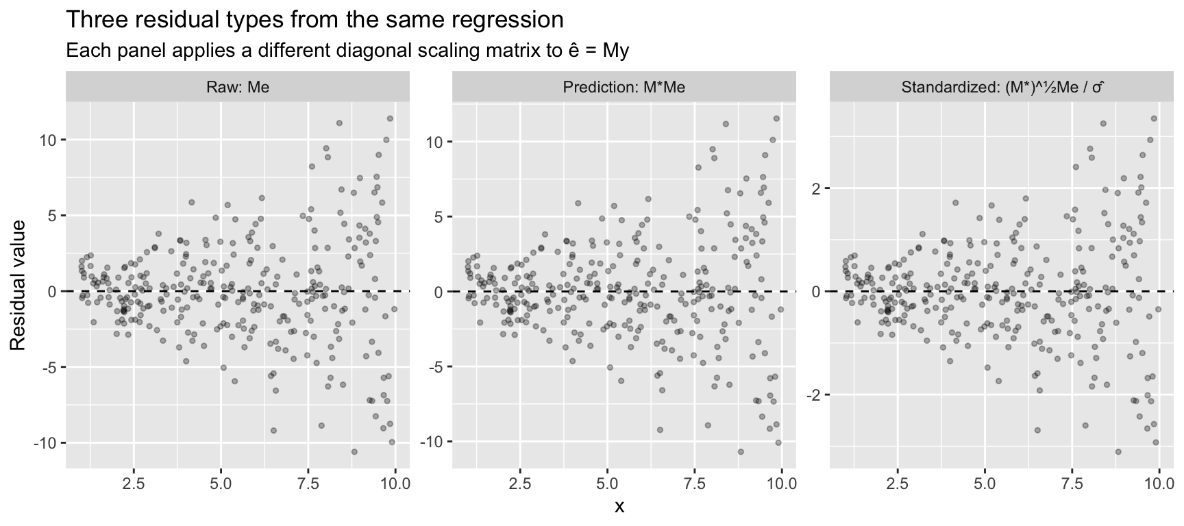
The fan shape is visible in all three (because the true DGP is heteroskedastic), but the scale differs: raw residuals have variance \((1 - h_{ii})\sigma_i^2\), prediction errors have variance \((1 - h_{ii})^{-1}\sigma_i^2\), and standardized residuals remove the leverage component, leaving only the heteroskedasticity \(\sigma_i^2 / \sigma^2\).
Studentized residuals. R also provides rstudent(), which replaces \(\hat{\sigma}\) with the leave-one-out estimate \(s_{(-i)}\). In practice, studentized and standardized residuals are nearly identical for moderate \(n\) — the difference is just one observation’s contribution to \(\hat{\sigma}^2\). The studentized version follows a \(t_{n-K-1}\) distribution under normality, which is useful for formal outlier tests:
# Studentized ≈ standardized, but uses leave-one-out sigma
max(abs(rstudent(mod_diag) - rstandard(mod_diag)))
[1] 0.0597 Bootstrap and permutation inference
The sandwich estimators (HC0–HC3) are analytical corrections — they adjust the standard error formula using leverage and squared residuals. Bootstrap and permutation methods take a different approach: they estimate the sampling distribution directly by resampling the data. No formula for \(\Omega\) is needed.
7.1 Pairs bootstrap
The simplest bootstrap resamples rows of \((y_i, x_i)\) with replacement and re-estimates \(\hat\beta\) each time. The standard deviation of the bootstrap distribution estimates the standard error:
set.seed(42)
B_boot <- 2000
beta_boot <- numeric(B_boot)

for (b in 1:B_boot) {
  idx <- sample(n, replace = TRUE)
  beta_boot[b] <- coef(lm(y[idx] ~ x[idx]))[2]
}

se_boot_pairs <- sd(beta_boot)
The pairs bootstrap is robust to heteroskedasticity because each resample inherits the variance structure of the original data — high-variance observations naturally appear with their high variance.
7.2 Wild bootstrap
The wild bootstrap is designed specifically for heteroskedastic regression. Instead of resampling rows, it keeps \(X\) fixed and generates new responses by multiplying the residuals by random signs:
\[y_i^* = \hat{y}_i + \frac{\hat{e}_i}{\sqrt{1 - h_{ii}}} \cdot v_i, \quad v_i \stackrel{iid}{\sim} \text{Rademacher}(\pm 1)\]
The \(1/\sqrt{1-h_{ii}}\) correction (the same leverage adjustment behind HC2) ensures the resampled errors have the right conditional variance.
set.seed(42)
fitted_vals <- fitted(mod_diag)
e_scaled <- resid(mod_diag) / sqrt(1 - h)

beta_wild <- numeric(B_boot)
for (b in 1:B_boot) {
  v <- sample(c(-1, 1), n, replace = TRUE)  # Rademacher weights
  y_star <- fitted_vals + e_scaled * v
  beta_wild[b] <- coef(lm(y_star ~ x))[2]
}

se_boot_wild <- sd(beta_wild)
7.3 Permutation test
A permutation test asks a different question: under the sharp null hypothesis that \(\beta_1 = 0\) (i.e., \(y\) is unrelated to \(x\)), how extreme is the observed coefficient? Under the null, the pairing of \(y_i\) with \(x_i\) is arbitrary, so we can shuffle \(y\) and recompute \(\hat\beta\) to build a null distribution.
set.seed(42)
B_perm <- 5000
beta_obs <- coef(mod_diag)[2]
beta_perm <- numeric(B_perm)

for (b in 1:B_perm) {
  y_perm <- sample(y)  # break the (y, x) pairing
  beta_perm[b] <- coef(lm(y_perm ~ x))[2]
}

p_perm <- mean(abs(beta_perm) >= abs(beta_obs))
The permutation p-value is exact under the null — no distributional assumptions required. But note two limitations: the permutation test targets the sharp null (\(y_i \perp\!\!\!\perp x_i\), not just \(\beta = 0\)), and it does not naturally produce confidence intervals (though inversion is possible).
7.4 Comparing all approaches
se_classical <- summary(mod_diag)$coefficients[2, 2]
se_hc3 <- sqrt(vcovHC(mod_diag, type = "HC3")[2, 2])

se_compare_all <- data.frame(
  method = c("Classical", "HC3 (jackknife)", "Pairs bootstrap",
             "Wild bootstrap", "Permutation"),
  SE = round(c(se_classical, se_hc3, se_boot_pairs,
               se_boot_wild, NA), 4),
  p_value = formatC(c(
    summary(mod_diag)$coefficients[2, 4],
    coeftest(mod_diag, vcov = vcovHC(mod_diag, type = "HC3"))[2, 4],
    # Bootstrap p-values: fraction of bootstrap dist. beyond zero (two-sided)
    2 * min(mean(beta_boot >= 0), mean(beta_boot <= 0)),
    2 * min(mean(beta_wild >= 0), mean(beta_wild <= 0)),
    p_perm
  ), format = "g", digits = 3)
)
se_compare_all
method SE p_value
1 Classical 0.0753 3.71e-122
2 HC3 (jackknife) 0.0891 2.65e-104
3 Pairs bootstrap 0.0861 0
4 Wild bootstrap 0.0886 0
5 Permutation NA 0The approaches differ in what they assume:
| Method | Assumes | Gives SEs? | Gives p-values? |
|---|---|---|---|
| Classical | Homoskedasticity, normality | Yes | Yes |
| HC3 (jackknife) | Nothing about \(\Omega\) | Yes | Yes |
| Pairs bootstrap | \((y_i, x_i)\) are iid | Yes (SD of bootstrap dist.) | Yes (percentile) |
| Wild bootstrap | \(X\) fixed, heteroskedastic errors | Yes | Yes |
| Permutation | Sharp null: \(y \perp\!\!\!\perp x\) | No (by default) | Yes (exact) |
For cross-sectional linear regression with heteroskedasticity, HC3 and the wild bootstrap are the most appropriate. The pairs bootstrap is simple and widely used but can undercover in small samples with high leverage. The permutation test is assumption-free but answers a narrower question. We return to bootstrap methods in Chapter 8 (Asymptotics).
8 Estimating \(\sigma^2\)
Three estimators of the error variance:
K <- ncol(X_d)

# 1. Method of moments (biased)
sigma2_mm <- sum(resid(mod_diag)^2) / n

# 2. Bias-corrected (used by summary.lm)
sigma2_s2 <- sum(resid(mod_diag)^2) / (n - K)

# 3. Standardized estimator (unbiased under heteroskedasticity)
sigma2_bar <- mean(resid(mod_diag)^2 / (1 - h))

c(MM = sigma2_mm, s2 = sigma2_s2, standardized = sigma2_bar)
MM s2 standardized
11.6 11.7 11.7 Under homoskedasticity, \(s^2\) is unbiased: \(E[s^2 \mid X] = \sigma^2\). The key identity is \(E[\hat{e}'\hat{e} \mid X] = \text{tr}(M) \cdot \sigma^2 = (n - K)\sigma^2\).
# The trace trick: E[e'Me] = tr(M * E[ee']) = tr(M) * sigma^2 under homoskedasticity
c(trace_M = tr(M_d), n_minus_K = n - K)
trace_M n_minus_K
298 298 The standardized estimator \(\bar{\sigma}^2 = \frac{1}{n}\sum (1-h_{ii})^{-1}\hat{e}_i^2\) is unbiased even under heteroskedasticity — it corrects each squared residual for its leverage. This is the logic behind HC2 standard errors: replace \(\hat{e}_i^2\) with \(\hat{e}_i^2 / (1 - h_{ii})\) in the sandwich meat. HC3 goes further, using \(\hat{e}_i^2 / (1 - h_{ii})^2\) — the extra factor makes it equivalent to the jackknife and more conservative at high-leverage points.
9 Hansen’s \(\tilde{R}^2\): cross-validated fit
The standard \(R^2 = 1 - \text{SSE}/\text{SST}\) measures in-sample fit: how well does the model predict the data it was trained on? This is biased upward — adding regressors always increases \(R^2\), even if they are pure noise. The adjusted \(R^2\) applies a degrees-of-freedom correction, but it is still based on in-sample residuals \(\hat{e}_i\).
Hansen recommends a more honest measure: replace the in-sample residuals with the prediction errors (leave-one-out residuals) \(\tilde{e}_i = \hat{e}_i / (1 - h_{ii})\). These are the same prediction errors from Section 6 — each \(\tilde{e}_i\) is the error you would make predicting observation \(i\) from a model fit without observation \(i\).
\[\tilde{R}^2 = 1 - \frac{\sum_{i=1}^n \tilde{e}_i^2}{\sum_{i=1}^n (Y_i - \bar{Y})^2} \tag{4}\]
This is a cross-validated \(R^2\). It penalizes overfitting more aggressively than adjusted \(R^2\) because prediction errors \(\tilde{e}_i\) are always larger than in-sample residuals — the model had access to observation \(i\) when computing \(\hat{e}_i\), but not when computing \(\tilde{e}_i\). Unlike regular \(R^2\), \(\tilde{R}^2\) can be negative if the model overfits so badly that it predicts worse than the sample mean.
Here is a reusable R function:
r2_tilde <- function(mod) {
  e_hat <- resid(mod)
  h <- hatvalues(mod)
  e_tilde <- e_hat / (1 - h)           # prediction errors
  y <- mod$model[[1]]                   # response variable
  SST <- sum((y - mean(y))^2)
  1 - sum(e_tilde^2) / SST
}
Let’s compare it to \(R^2\) and adjusted \(R^2\) on the Prestige data:
mod_p <- lm(prestige ~ education + income + women, data = Prestige)

c(R2         = summary(mod_p)$r.squared,
  adj_R2     = summary(mod_p)$adj.r.squared,
  tilde_R2   = r2_tilde(mod_p))
R2 adj_R2 tilde_R2
0.798 0.792 0.777 Now watch what happens when we add noise regressors — variables that are pure random noise with no relationship to prestige:
set.seed(42)
Prestige$noise1 <- rnorm(nrow(Prestige))
Prestige$noise2 <- rnorm(nrow(Prestige))
Prestige$noise3 <- rnorm(nrow(Prestige))

mod_noise <- lm(prestige ~ education + income + women +
                  noise1 + noise2 + noise3, data = Prestige)

comparison <- data.frame(
  baseline = c(summary(mod_p)$r.squared,
               summary(mod_p)$adj.r.squared,
               r2_tilde(mod_p)),
  with_noise = c(summary(mod_noise)$r.squared,
                 summary(mod_noise)$adj.r.squared,
                 r2_tilde(mod_noise)),
  row.names = c("R²", "Adjusted R²", "R² tilde (Hansen)")
)
round(comparison, 4)
baseline with_noise
R² 0.798 0.801
Adjusted R² 0.792 0.788
R² tilde (Hansen) 0.777 0.766Regular \(R^2\) goes up (it always does). Adjusted \(R^2\) goes down slightly. Hansen’s \(\tilde{R}^2\) drops more sharply — it reflects the fact that out-of-sample prediction has gotten worse by fitting noise.
TipReporting Fit
Following Hansen, report \(\tilde{R}^2\) alongside or in place of adjusted \(R^2\). It gives a more honest assessment of predictive fit because it is based on leave-one-out prediction errors, not in-sample residuals. Compute it with r2_tilde(mod) defined above.
10 Method of moments perspective
10.1 OLS as a method of moments estimator
OLS solves the sample analog of \(E[x_i(y_i - x_i'\beta)] = 0\):
\[\frac{1}{n} \sum_{i=1}^n x_i(y_i - x_i'\hat{\beta}) = 0 \quad \Longleftrightarrow \quad X'(y - X\hat{\beta}) = 0\]
# The OLS normal equations are moment conditions
moment <- t(X_d) %*% resid(mod_diag)
moment  # numerically zero
[,1]
2.78e-15
x 5.62e-1310.2 GLS as efficient method of moments
GLS solves a weighted version of the same moment condition:
\[\frac{1}{n} \sum_{i=1}^n \frac{1}{\sigma_i^2} x_i(y_i - x_i'\hat{\beta}_{GLS}) = 0 \quad \Longleftrightarrow \quad X'\Omega^{-1}(y - X\hat{\beta}_{GLS}) = 0\]
This is a generalized method of moments (GMM) estimator with weight matrix \(\Omega^{-1}\).
# GLS normal equations
Omega_hat_inv_diag <- diag(1 / sigma2_hat)  # from our FGLS above
moment_gls <- t(X_d) %*% Omega_hat_inv_diag %*% resid(mod_fgls)
moment_gls  # numerically zero
[,1]
1.11e-14
x -2.22e-14When we have exactly as many moment conditions as parameters (\(K\) equations, \(K\) unknowns), the GMM estimator reduces to method of moments. The efficiency of GLS comes from choosing the optimal weight matrix.
In Chapter 14, we’ll see that this logic extends to overidentified models: when you have more moment conditions than parameters, GMM finds the optimal combination. The GLS insight — weight by precision — is the same insight that drives GMM.
11 Application: robust inference on the Prestige data
Let’s apply the practical workflow to the Prestige dataset. We start with lm_robust() as the default — no pre-testing required.
# The default workflow: OLS with HC3 robust SEs
mod_p_robust <- lm_robust(prestige ~ education + income + women,
                           data = Prestige, se_type = "HC3")
summary(mod_p_robust)
Call:
lm_robust(formula = prestige ~ education + income + women, data = Prestige,
    se_type = "HC3")

Standard error type:  HC3

Coefficients:
            Estimate Std. Error t value Pr(>|t|)  CI Lower CI Upper DF
(Intercept) -6.79433   3.293972  -2.063 4.18e-02 -1.33e+01 -0.25755 98
education    4.18664   0.479553   8.730 6.85e-14  3.23e+00  5.13829 98
income       0.00131   0.000421   3.117 2.40e-03  4.77e-04  0.00215 98
women       -0.00891   0.037558  -0.237 8.13e-01 -8.34e-02  0.06563 98

Multiple R-squared:  0.798 ,    Adjusted R-squared:  0.792
F-statistic:  126 on 3 and 98 DF,  p-value: <2e-16
That’s the complete inference in one line. The residual plot is still useful as a descriptive tool for understanding your data — it just shouldn’t gate your choice of estimator:
mod_p <- lm(prestige ~ education + income + women, data = Prestige)
df_p <- data.frame(income = Prestige$income, resid = resid(mod_p))
ggplot(df_p, aes(income, resid)) +
  geom_point(alpha = 0.5) +
  geom_hline(yintercept = 0, linetype = "dashed") +
  geom_smooth(se = FALSE, color = "steelblue", method = "loess", formula = y ~ x) +
  labs(title = "Prestige: residuals vs. income",
       subtitle = "Useful for understanding the data, not for choosing an estimator")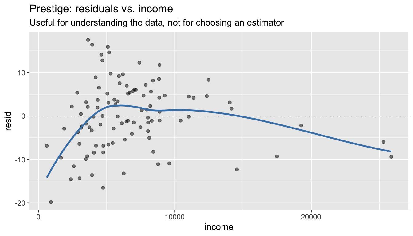
For comparison, here is what FGLS would give if we had a substantive reason to believe variance is proportional to income (e.g., because occupational prestige surveys sample more respondents for common jobs):
# FGLS: only if we have a theoretical reason for the variance model
log_e2_p <- log(resid(mod_p)^2)
mod_var_p <- lm(log_e2_p ~ income, data = Prestige)
sigma2_hat_p <- exp(fitted(mod_var_p))

mod_fgls_p <- lm(prestige ~ education + income + women,
                  data = Prestige, weights = 1 / sigma2_hat_p)
# Full comparison: coefficients and standard errors
coefs <- cbind(
OLS = coef(mod_p),
HC3 = coef(mod_p), # same point estimates
FGLS = coef(mod_fgls_p) # different point estimates
)
ses <- cbind(
Classical = summary(mod_p)$coefficients[, 2],
HC3 = summary(mod_p_robust)$coefficients[, 2],
FGLS = summary(mod_fgls_p)$coefficients[, 2]
)
cat("Point estimates:\n")Point estimates:round(coefs, 4) OLS HC3 FGLS
(Intercept) -6.7943 -6.7943 -6.6482
education 4.1866 4.1866 4.2360
income 0.0013 0.0013 0.0012
women -0.0089 -0.0089 -0.0132cat("\nStandard errors:\n")
Standard errors:round(ses, 4) Classical HC3 FGLS
(Intercept) 3.2391 3.2940 3.2241
education 0.3887 0.4796 0.3816
income 0.0003 0.0004 0.0003
women 0.0304 0.0376 0.0302The differences here are modest. The pattern illustrates the two strategies:
- Robust SEs (HC3): Keep the OLS point estimates, correct only the standard errors. No assumptions about the variance structure — always valid.
- FGLS: Re-estimate \(\hat{\beta}\) using the variance structure. More efficient if your variance model is correct; potentially worse if it’s wrong.
The default for linear regression is HC3. Use FGLS when you have a substantive reason to model the variance — not because a test told you to.
TipHC3 as Default for Linear Regression
For linear regression, use lm_robust(y ~ x, se_type = "HC3") or vcovHC(mod, type = "HC3") as the default. HC3 is equivalent to the jackknife variance estimator and provides the best finite-sample coverage among the HC variants. Note that estimatr defaults to HC2 — pass se_type = "HC3" explicitly.
12 Summary
| Concept | Matrix formula | R code |
|---|---|---|
| Sandwich variance | \((X'X)^{-1}X'\Omega X(X'X)^{-1}\) | vcovHC(mod, type = "HC3") |
| Robust SEs | \(\sqrt{\text{diag}(\hat{V}_{HC})}\) | lm_robust(y ~ x, se_type = "HC3") |
| Robust t-test | — | coeftest(mod, vcov = vcovHC) |
| WLS | \((X'WX)^{-1}X'Wy\) | lm(y ~ x, weights = w) |
| GLS | \((X'\Omega^{-1}X)^{-1}X'\Omega^{-1}y\) | solve(t(X) %*% Oi %*% X) %*% t(X) %*% Oi %*% y |
| Eigendecomposition | \(\Omega = C\Lambda C'\) | eigen(Omega) |
| \(\Omega^{-1/2}\) | \(C\Lambda^{-1/2}C'\) | C %*% diag(1/sqrt(lam)) %*% t(C) |
| FGLS | Estimate \(\hat{\Omega}\), then GLS | lm(log(e^2) ~ z) then lm(y ~ x, weights = ...) |
| Breusch-Pagan | \(nR^2\) from \(\hat{e}^2/\bar{\hat{e}^2} \sim X\) | bptest(mod) |
| Standardized residual | \(\hat{e}_i / (\hat{\sigma}\sqrt{1-h_{ii}})\) | rstandard(mod) |
| Studentized residual | \(\hat{e}_i / (s_{(-i)}\sqrt{1-h_{ii}})\) | rstudent(mod) |
Key takeaway. When you know (or can estimate) the variance structure, exploit it: WLS/GLS gives you tighter estimates by trusting precise observations more. When you don’t trust your variance model, use lm_robust(..., se_type = "HC3") — the jackknife-based HC3 provides the best finite-sample coverage for linear regression and requires no assumptions about the form of heteroskedasticity. In either case, the method of moments logic — choosing the right weight matrix — connects directly to GMM (Chapter 14).